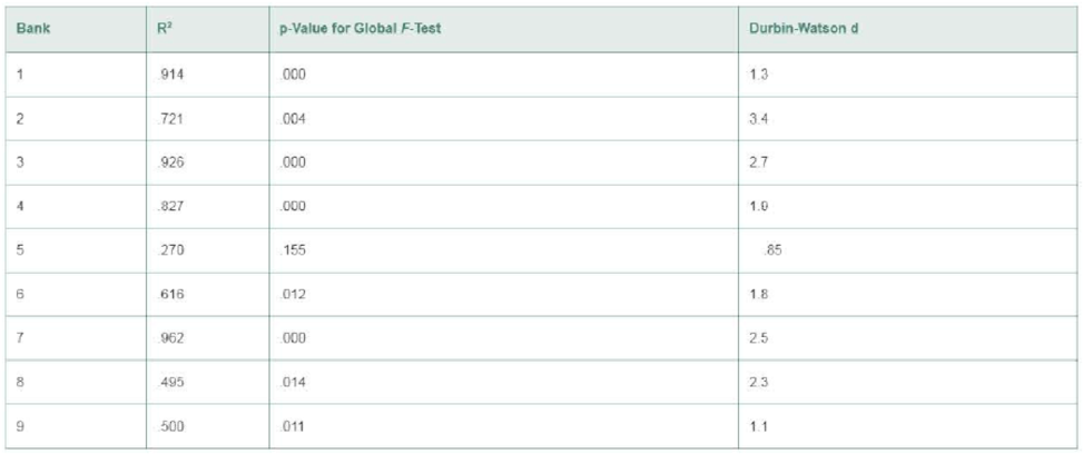
Modeling the deposit share of a retail bank. Exploratory research published in the Journal of Professional Services Marketing (Vol. 5, 1990) examined the relationship between deposit share of a retail bank and several marketing variables. Quarterly deposit share data were collected for 5 consecutive years for each of nine retail banking institutions. The model analyzed took the following form:
E(Yt) = β0 + β1Pt−1 + β2St−1 + β3Dt−1
where Yt = deposit share of a bank In quarter t (t = 1, 2, ... , 20), Pt−1 = expenditures on promotion-related activities in quarter t – 1, St−1 = expenditures on service- related activities in quarter t − 1, and Dt−1 = expenditures on distribution-related activities in quarter t – 1. A separate model was fit for each bank with the results shown in the table.
a. Interpret the values of R2 for each bank.
b. Test the overall adequacy of the model for each bank using α = .01.
c. Conduct the Durbin-Watson d-test for

Want to see the full answer?
Check out a sample textbook solution
Chapter 14 Solutions
Statistics for Business and Economics (13th Edition)
- We have data on Lung Capacity of persons and we wish to build a multiple linear regression model that predicts Lung Capacity based on the predictors Age and Smoking Status. Age is a numeric variable whereas Smoke is a categorical variable (0 if non-smoker, 1 if smoker). Here is the partial result from STATISTICA. b* Std.Err. of b* Std.Err. N=725 of b Intercept Age Smoke 0.835543 -0.075120 1.085725 0.555396 0.182989 0.014378 0.021631 0.021631 -0.648588 0.186761 Which of the following statements is absolutely false? A. The expected lung capacity of a smoker is expected to be 0.648588 lower than that of a non-smoker. B. The predictor variables Age and Smoker both contribute significantly to the model. C. For every one year that a person gets older, the lung capacity is expected to increase by 0.555396 units, holding smoker status constant. D. For every one unit increase in smoker status, lung capacity is expected to decrease by 0.648588 units, holding age constant.arrow_forwardIn a simple linear regression model, the correlation coefficient between x and y is 0.8. What can you say about the strength and direction of the relationship between x and y?arrow_forwardA study was conducted to see if a person's income will affect their well-being. We want to create a model with Y = well-being index, and X = income in $1,000. The dependent variable in this study is: Income in $1,000 Well-being index Neitherarrow_forward
- Look at the following regression table where the dependent variable is the demand for illegal massage services in a city in the United States. Specifically, the dependent variable is the number of customers per hour (Models 1 and 2) or per day (Models 3 and 4). (a) Explain why the coefficient for Population/1,000 in Model 2 is very different from the one in Model 4?(b) Can you reject H0 in Model 1 if H0 : βP opulation/1,000 = 0.01, H1 : βPopulation/1,000 6= 0.01, and α = 0.01?arrow_forwardWhy would the male lifespan not be the dependent variable?arrow_forwardAssume we have data demonstrating a strong linear link between the amount of fertilizer applied to certain plants and their yield. Which is the independent variable in this research question?arrow_forward
- I set up a multiple linear regression model to explain returns on BA as a linear function of market returns, and size and value. Note that the data is in levels ( not in logs) I interpret the beta of market as Select one: a. the impact of a one unit variation of market on BA returns on average b. the impact of a one unit % chnage in market on the BA returns on average keeping size and value fixed c. the relation between BA returns and market d. the impact of a one percentage variation of market on BA returns on average in percentage e. the impact of a one unit variation in market on the BA returns on average keeping size and value fixedarrow_forwardA regression was run to determine if there is a relationship between the happiness index (y) and life expectancy in years of a given country (x). The results of the regression were: ý=a+bx a=0.137 b=0.082 (a) Write the equation of the Least Squares Regression line of the form (b) Which is a possible value for the correlation coefficient, r? O-1.338 O-0.84 O 1.338 O 0.84 (c) If a country increases its life expectancy, the happiness index will O increase O decreasearrow_forwardIn the simple linear regression model, if there is a very strong correlation between the independent and dependent variables, then the correlation coefficient should be a) close to either -1 or +1 b) close to zero c) close to -1 d) close to +1 ( don't hand writing solution)arrow_forward
- A major brokerage company has an office in Miami, Florida. The manager of the office is evaluated based on the number of new clients generated each quarter. Data were collected that show the number of new customers added during each quarter between 2015 and 2018. A multiple regression model was developed with the number of new customers as the dependent and the following four independent variables: Period (1, …, 16): A variable that measures the trend; Q1 = 1 for first quarter, Q1 = 0 otherwise; Q2 = 1 for second quarter, Q2 = 0 otherwise; Q3 = 1 for third quarter, Q3 = 0 otherwise. Questions: 1. Explain each of the four slopes (Period, Q1, Q2, Q3). 2. How many new customers would you expect in the second quarter of the following year (2019)?arrow_forwardCaterpillar, Inc., manufactures and sells heavy construction equipment worldwide. The performance of Caterpillar’s stock is likely to be strongly influenced by the economy. For example, during the Great Recession, the value of Caterpillar’s stock plunged dramatically. Monthly data for Caterpillar’s risk-adjusted return (R − Rf) and the risk-adjusted market return (RM − Rf) are collected for a five-year period (n = 60). A portion of the data is shown in the accompanying table. (You may find it useful to reference the t table.) Month Year R_Rf RM_Rf Jan 2012 0.0510 0.0403 Feb 2012 -0.0682 0.0304 Mar 2012 -0.0360 -0.0083 Apr 2012 -0.1446 -0.0635 May 2012 -0.0318 0.0387 Jun 2012 -0.0091 0.0117 Jul 2012 0.0188 0.0188 Aug 2012 0.0073 0.0232 Sept 2012 -0.0154 -0.0209 Oct 2012 0.0101 0.0018 Nov 2012 0.0504 0.0062 Dec 2012 0.1036 0.0497 Jan 2013 -0.0619 0.0104 Feb 2013 -0.0595 0.0350 Mar 2013 -0.0273 0.0172 Apr 2013 0.0193 0.0202 May 2013 -0.0390 -0.0154…arrow_forwardDistress in EMSworkers. The Journal consulting and Clinical Psychology reported on a study of emergency service (EMS) rescue workers who responded to the I-880 freeway collapse during a San Francisco earthquake. The goal of the study was to identify the predictors of symptomatic distress in the EMS workers. One of the distress variables studied was the Global Symptom Index (GSI). Several models for GSI, y, were considered based on the following independent variables: x1 = Critical Incident Exposure scale (CIE) x2 = Hogan Personality Inventory—Adjustment scale (HPI-A) x3 = Years of experience (EXP) x4 = Locus of Control scale (LOC) x5 = Social Support scale (SS) x6 = Dissociative Experiences scale (DES) x7 = Peritraumatic Dissociation Experiences Questionnaire, self-report (PDEQ-SR) (a) Write a first-order model for E(y) as a function of the first five independent variables, x1 –x5. (b) The model of part a, fitted to data collected for n = 147 EMS workers, yielded the following results:…arrow_forward
 Glencoe Algebra 1, Student Edition, 9780079039897...AlgebraISBN:9780079039897Author:CarterPublisher:McGraw Hill
 Big Ideas Math A Bridge To Success Algebra 1: Stu...AlgebraISBN:9781680331141Author:HOUGHTON MIFFLIN HARCOURTPublisher:Houghton Mifflin Harcourt


