Concept explainers
Videos
a.
To find:The regression equation for the data.
a.
Answer to Problem 21E
The regression equation for the data is
Explanation of Solution
Given information: The data is shown below.
| 31.3 | 50 | 19 | 4.0 | 37.4 | 60 | 30 | 5.0 | 24.0 | 60 | 24 | 4.0 | 51.0 | 80 | 34 | 7.5 |
| 56.9 | 90 | 38 | 8.0 | 43.3 | 60 | 26 | 7.0 | 36.2 | 50 | 21 | 7.0 | 34.3 | 60 | 22 | 2.5 |
| 43.1 | 70 | 28 | 6.5 | 36.3 | 70 | 25 | 7.5 | 26.5 | 50 | 17 | 2.0 | 31.5 | 60 | 24 | 5.0 |
| 41.5 | 70 | 25 | 5.5 | 38.4 | 70 | 31 | 5.5 | 47.1 | 80 | 34 | 8.5 | 33.2 | 60 | 23 | 4.0 |
| 39.0 | 60 | 26 | 6.5 | 41.5 | 60 | 27 | 7.5 | 38.1 | 70 | 27 | 5.5 | 39.2 | 60 | 29 | 6.5 |
| 40.9 | 70 | 29 | 5.0 | 36.l | 60 | 23 | 6.0 | 33.5 | 60 | 24 | 2.5 | 46.7 | 70 | 27 | 7.5 |
| 35.9 | 60 | 23 | 5.5 | 38.5 | 60 | 23 | 6.0 | 43.6 | 70 | 27 | 10.0 | 30.4 | 70 | 32 | 4.0 |
| 43.5 | 70 | 28 | 5.5 | 42.4 | 60 | 24 | 9.0 | 41.0 | 80 | 32 | 6.5 | 43.2 | 60 | 25 | 5.5 |
| 47.9 | 80 | 34 | 6.5 | 46.5 | 70 | 31 | 5.5 | 50.2 | 50 | 26 | 9.0 | 30.6 | 60 | 26 | 3.5 |
| 33.8 | 70 | 26 | 4.5 | 43.1 | 80 | 32 | 6.0 | 34.4 | 50 | 22 | 4.0 | 43.3 | 70 | 28 | 7.5 |
| 41.1 | 70 | 26 | 8.0 | 50.8 | 60 | 26 | 10.0 | 47.9 | 80 | 34 | 6.5 | 32.4 | 60 | 22 | 5.5 |
| 38.7 | 70 | 26 | 8.0 | 44.2 | 70 | 28 | 4.5 | 46.2 | 50 | 21 | 10.0 | 35.5 | 60 | 22 | 4.5 |
Calculation:
The MINITAB is shown below,
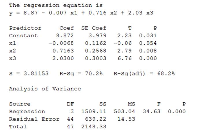
Figure-1
From Figure-1 it is clear that the regression equation is
b.
To find: The value of variable
b.
Answer to Problem 21E
The value of variable
Explanation of Solution
Given information: The data is shown below.
| 31.3 | 50 | 19 | 4.0 | 37.4 | 60 | 30 | 5.0 | 24.0 | 60 | 24 | 4.0 | 51.0 | 80 | 34 | 7.5 |
| 56.9 | 90 | 38 | 8.0 | 43.3 | 60 | 26 | 7.0 | 36.2 | 50 | 21 | 7.0 | 34.3 | 60 | 22 | 2.5 |
| 43.1 | 70 | 28 | 6.5 | 36.3 | 70 | 25 | 7.5 | 26.5 | 50 | 17 | 2.0 | 31.5 | 60 | 24 | 5.0 |
| 41.5 | 70 | 25 | 5.5 | 38.4 | 70 | 31 | 5.5 | 47.1 | 80 | 34 | 8.5 | 33.2 | 60 | 23 | 4.0 |
| 39.0 | 60 | 26 | 6.5 | 41.5 | 60 | 27 | 7.5 | 38.1 | 70 | 27 | 5.5 | 39.2 | 60 | 29 | 6.5 |
| 40.9 | 70 | 29 | 5.0 | 36.l | 60 | 23 | 6.0 | 33.5 | 60 | 24 | 2.5 | 46.7 | 70 | 27 | 7.5 |
| 35.9 | 60 | 23 | 5.5 | 38.5 | 60 | 23 | 6.0 | 43.6 | 70 | 27 | 10.0 | 30.4 | 70 | 32 | 4.0 |
| 43.5 | 70 | 28 | 5.5 | 42.4 | 60 | 24 | 9.0 | 41.0 | 80 | 32 | 6.5 | 43.2 | 60 | 25 | 5.5 |
| 47.9 | 80 | 34 | 6.5 | 46.5 | 70 | 31 | 5.5 | 50.2 | 50 | 26 | 9.0 | 30.6 | 60 | 26 | 3.5 |
| 33.8 | 70 | 26 | 4.5 | 43.1 | 80 | 32 | 6.0 | 34.4 | 50 | 22 | 4.0 | 43.3 | 70 | 28 | 7.5 |
| 41.1 | 70 | 26 | 8.0 | 50.8 | 60 | 26 | 10.0 | 47.9 | 80 | 34 | 6.5 | 32.4 | 60 | 22 | 5.5 |
| 38.7 | 70 | 26 | 8.0 | 44.2 | 70 | 28 | 4.5 | 46.2 | 50 | 21 | 10.0 | 35.5 | 60 | 22 | 4.5 |
Calculation:
From Figure-1 it is clear that the regression equation is
Substitute the values in above equation.
Thus, the value of variable
c.
To find: The confidence interval.
c.
Answer to Problem 21E
The confidence intervalis
Explanation of Solution
Given information: The data is shown below.
| 31.3 | 50 | 19 | 4.0 | 37.4 | 60 | 30 | 5.0 | 24.0 | 60 | 24 | 4.0 | 51.0 | 80 | 34 | 7.5 |
| 56.9 | 90 | 38 | 8.0 | 43.3 | 60 | 26 | 7.0 | 36.2 | 50 | 21 | 7.0 | 34.3 | 60 | 22 | 2.5 |
| 43.1 | 70 | 28 | 6.5 | 36.3 | 70 | 25 | 7.5 | 26.5 | 50 | 17 | 2.0 | 31.5 | 60 | 24 | 5.0 |
| 41.5 | 70 | 25 | 5.5 | 38.4 | 70 | 31 | 5.5 | 47.1 | 80 | 34 | 8.5 | 33.2 | 60 | 23 | 4.0 |
| 39.0 | 60 | 26 | 6.5 | 41.5 | 60 | 27 | 7.5 | 38.1 | 70 | 27 | 5.5 | 39.2 | 60 | 29 | 6.5 |
| 40.9 | 70 | 29 | 5.0 | 36.l | 60 | 23 | 6.0 | 33.5 | 60 | 24 | 2.5 | 46.7 | 70 | 27 | 7.5 |
| 35.9 | 60 | 23 | 5.5 | 38.5 | 60 | 23 | 6.0 | 43.6 | 70 | 27 | 10.0 | 30.4 | 70 | 32 | 4.0 |
| 43.5 | 70 | 28 | 5.5 | 42.4 | 60 | 24 | 9.0 | 41.0 | 80 | 32 | 6.5 | 43.2 | 60 | 25 | 5.5 |
| 47.9 | 80 | 34 | 6.5 | 46.5 | 70 | 31 | 5.5 | 50.2 | 50 | 26 | 9.0 | 30.6 | 60 | 26 | 3.5 |
| 33.8 | 70 | 26 | 4.5 | 43.1 | 80 | 32 | 6.0 | 34.4 | 50 | 22 | 4.0 | 43.3 | 70 | 28 | 7.5 |
| 41.1 | 70 | 26 | 8.0 | 50.8 | 60 | 26 | 10.0 | 47.9 | 80 | 34 | 6.5 | 32.4 | 60 | 22 | 5.5 |
| 38.7 | 70 | 26 | 8.0 | 44.2 | 70 | 28 | 4.5 | 46.2 | 50 | 21 | 10.0 | 35.5 | 60 | 22 | 4.5 |
Calculation:
The MINITAB output is shown below.
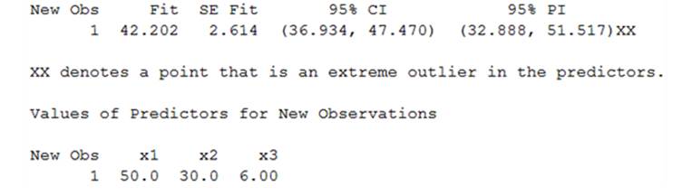
Figure-2
From Figure-2 it is clear that the confidence interval is
d.
To find: The prediction interval.
d.
Answer to Problem 21E
The prediction intervalis
Explanation of Solution
Given information: The data is shown below.
| 31.3 | 50 | 19 | 4.0 | 37.4 | 60 | 30 | 5.0 | 24.0 | 60 | 24 | 4.0 | 51.0 | 80 | 34 | 7.5 |
| 56.9 | 90 | 38 | 8.0 | 43.3 | 60 | 26 | 7.0 | 36.2 | 50 | 21 | 7.0 | 34.3 | 60 | 22 | 2.5 |
| 43.1 | 70 | 28 | 6.5 | 36.3 | 70 | 25 | 7.5 | 26.5 | 50 | 17 | 2.0 | 31.5 | 60 | 24 | 5.0 |
| 41.5 | 70 | 25 | 5.5 | 38.4 | 70 | 31 | 5.5 | 47.1 | 80 | 34 | 8.5 | 33.2 | 60 | 23 | 4.0 |
| 39.0 | 60 | 26 | 6.5 | 41.5 | 60 | 27 | 7.5 | 38.1 | 70 | 27 | 5.5 | 39.2 | 60 | 29 | 6.5 |
| 40.9 | 70 | 29 | 5.0 | 36.l | 60 | 23 | 6.0 | 33.5 | 60 | 24 | 2.5 | 46.7 | 70 | 27 | 7.5 |
| 35.9 | 60 | 23 | 5.5 | 38.5 | 60 | 23 | 6.0 | 43.6 | 70 | 27 | 10.0 | 30.4 | 70 | 32 | 4.0 |
| 43.5 | 70 | 28 | 5.5 | 42.4 | 60 | 24 | 9.0 | 41.0 | 80 | 32 | 6.5 | 43.2 | 60 | 25 | 5.5 |
| 47.9 | 80 | 34 | 6.5 | 46.5 | 70 | 31 | 5.5 | 50.2 | 50 | 26 | 9.0 | 30.6 | 60 | 26 | 3.5 |
| 33.8 | 70 | 26 | 4.5 | 43.1 | 80 | 32 | 6.0 | 34.4 | 50 | 22 | 4.0 | 43.3 | 70 | 28 | 7.5 |
| 41.1 | 70 | 26 | 8.0 | 50.8 | 60 | 26 | 10.0 | 47.9 | 80 | 34 | 6.5 | 32.4 | 60 | 22 | 5.5 |
| 38.7 | 70 | 26 | 8.0 | 44.2 | 70 | 28 | 4.5 | 46.2 | 50 | 21 | 10.0 | 35.5 | 60 | 22 | 4.5 |
Calculation:
From Figure-12 it is clear that the
e.
To find: The percentage of variation in variable
e.
Answer to Problem 21E
The percentage of variation in variable
Explanation of Solution
Given information: The data is shown below.
| 31.3 | 50 | 19 | 4.0 | 37.4 | 60 | 30 | 5.0 | 24.0 | 60 | 24 | 4.0 | 51.0 | 80 | 34 | 7.5 |
| 56.9 | 90 | 38 | 8.0 | 43.3 | 60 | 26 | 7.0 | 36.2 | 50 | 21 | 7.0 | 34.3 | 60 | 22 | 2.5 |
| 43.1 | 70 | 28 | 6.5 | 36.3 | 70 | 25 | 7.5 | 26.5 | 50 | 17 | 2.0 | 31.5 | 60 | 24 | 5.0 |
| 41.5 | 70 | 25 | 5.5 | 38.4 | 70 | 31 | 5.5 | 47.1 | 80 | 34 | 8.5 | 33.2 | 60 | 23 | 4.0 |
| 39.0 | 60 | 26 | 6.5 | 41.5 | 60 | 27 | 7.5 | 38.1 | 70 | 27 | 5.5 | 39.2 | 60 | 29 | 6.5 |
| 40.9 | 70 | 29 | 5.0 | 36.l | 60 | 23 | 6.0 | 33.5 | 60 | 24 | 2.5 | 46.7 | 70 | 27 | 7.5 |
| 35.9 | 60 | 23 | 5.5 | 38.5 | 60 | 23 | 6.0 | 43.6 | 70 | 27 | 10.0 | 30.4 | 70 | 32 | 4.0 |
| 43.5 | 70 | 28 | 5.5 | 42.4 | 60 | 24 | 9.0 | 41.0 | 80 | 32 | 6.5 | 43.2 | 60 | 25 | 5.5 |
| 47.9 | 80 | 34 | 6.5 | 46.5 | 70 | 31 | 5.5 | 50.2 | 50 | 26 | 9.0 | 30.6 | 60 | 26 | 3.5 |
| 33.8 | 70 | 26 | 4.5 | 43.1 | 80 | 32 | 6.0 | 34.4 | 50 | 22 | 4.0 | 43.3 | 70 | 28 | 7.5 |
| 41.1 | 70 | 26 | 8.0 | 50.8 | 60 | 26 | 10.0 | 47.9 | 80 | 34 | 6.5 | 32.4 | 60 | 22 | 5.5 |
| 38.7 | 70 | 26 | 8.0 | 44.2 | 70 | 28 | 4.5 | 46.2 | 50 | 21 | 10.0 | 35.5 | 60 | 22 | 4.5 |
Calculation:
From Figure-1 it is clear that the percentage of variation in variable
f.
To find:Whether the given model is useful for prediction.
f.
Answer to Problem 21E
The model is useful in prediction.
Explanation of Solution
Given information: The data is shown below.
| 31.3 | 50 | 19 | 4.0 | 37.4 | 60 | 30 | 5.0 | 24.0 | 60 | 24 | 4.0 | 51.0 | 80 | 34 | 7.5 |
| 56.9 | 90 | 38 | 8.0 | 43.3 | 60 | 26 | 7.0 | 36.2 | 50 | 21 | 7.0 | 34.3 | 60 | 22 | 2.5 |
| 43.1 | 70 | 28 | 6.5 | 36.3 | 70 | 25 | 7.5 | 26.5 | 50 | 17 | 2.0 | 31.5 | 60 | 24 | 5.0 |
| 41.5 | 70 | 25 | 5.5 | 38.4 | 70 | 31 | 5.5 | 47.1 | 80 | 34 | 8.5 | 33.2 | 60 | 23 | 4.0 |
| 39.0 | 60 | 26 | 6.5 | 41.5 | 60 | 27 | 7.5 | 38.1 | 70 | 27 | 5.5 | 39.2 | 60 | 29 | 6.5 |
| 40.9 | 70 | 29 | 5.0 | 36.l | 60 | 23 | 6.0 | 33.5 | 60 | 24 | 2.5 | 46.7 | 70 | 27 | 7.5 |
| 35.9 | 60 | 23 | 5.5 | 38.5 | 60 | 23 | 6.0 | 43.6 | 70 | 27 | 10.0 | 30.4 | 70 | 32 | 4.0 |
| 43.5 | 70 | 28 | 5.5 | 42.4 | 60 | 24 | 9.0 | 41.0 | 80 | 32 | 6.5 | 43.2 | 60 | 25 | 5.5 |
| 47.9 | 80 | 34 | 6.5 | 46.5 | 70 | 31 | 5.5 | 50.2 | 50 | 26 | 9.0 | 30.6 | 60 | 26 | 3.5 |
| 33.8 | 70 | 26 | 4.5 | 43.1 | 80 | 32 | 6.0 | 34.4 | 50 | 22 | 4.0 | 43.3 | 70 | 28 | 7.5 |
| 41.1 | 70 | 26 | 8.0 | 50.8 | 60 | 26 | 10.0 | 47.9 | 80 | 34 | 6.5 | 32.4 | 60 | 22 | 5.5 |
| 38.7 | 70 | 26 | 8.0 | 44.2 | 70 | 28 | 4.5 | 46.2 | 50 | 21 | 10.0 | 35.5 | 60 | 22 | 4.5 |
Calculation:
The null hypothesis is, the model is not useful for prediction and the alternative hypothesis is, the model is useful in prediction.
From Figure-1 it is clear that the p value is less than the level of significance of
Hence, the null hypothesis is rejected.
Thus, the model is useful in prediction.
g.
To explain:The test for the hypothesis
g.
Explanation of Solution
Given information: The data is shown below.
| 31.3 | 50 | 19 | 4.0 | 37.4 | 60 | 30 | 5.0 | 24.0 | 60 | 24 | 4.0 | 51.0 | 80 | 34 | 7.5 |
| 56.9 | 90 | 38 | 8.0 | 43.3 | 60 | 26 | 7.0 | 36.2 | 50 | 21 | 7.0 | 34.3 | 60 | 22 | 2.5 |
| 43.1 | 70 | 28 | 6.5 | 36.3 | 70 | 25 | 7.5 | 26.5 | 50 | 17 | 2.0 | 31.5 | 60 | 24 | 5.0 |
| 41.5 | 70 | 25 | 5.5 | 38.4 | 70 | 31 | 5.5 | 47.1 | 80 | 34 | 8.5 | 33.2 | 60 | 23 | 4.0 |
| 39.0 | 60 | 26 | 6.5 | 41.5 | 60 | 27 | 7.5 | 38.1 | 70 | 27 | 5.5 | 39.2 | 60 | 29 | 6.5 |
| 40.9 | 70 | 29 | 5.0 | 36.l | 60 | 23 | 6.0 | 33.5 | 60 | 24 | 2.5 | 46.7 | 70 | 27 | 7.5 |
| 35.9 | 60 | 23 | 5.5 | 38.5 | 60 | 23 | 6.0 | 43.6 | 70 | 27 | 10.0 | 30.4 | 70 | 32 | 4.0 |
| 43.5 | 70 | 28 | 5.5 | 42.4 | 60 | 24 | 9.0 | 41.0 | 80 | 32 | 6.5 | 43.2 | 60 | 25 | 5.5 |
| 47.9 | 80 | 34 | 6.5 | 46.5 | 70 | 31 | 5.5 | 50.2 | 50 | 26 | 9.0 | 30.6 | 60 | 26 | 3.5 |
| 33.8 | 70 | 26 | 4.5 | 43.1 | 80 | 32 | 6.0 | 34.4 | 50 | 22 | 4.0 | 43.3 | 70 | 28 | 7.5 |
| 41.1 | 70 | 26 | 8.0 | 50.8 | 60 | 26 | 10.0 | 47.9 | 80 | 34 | 6.5 | 32.4 | 60 | 22 | 5.5 |
| 38.7 | 70 | 26 | 8.0 | 44.2 | 70 | 28 | 4.5 | 46.2 | 50 | 21 | 10.0 | 35.5 | 60 | 22 | 4.5 |
The null hypothesis is, there is no relationship between
For the variable
From Figure-1 it is clear that the p value is
Hence, the null hypothesis is not rejected.
Thus, there is no linear relationship between
For the variable
From Figure-1 it is clear that the p value is
Hence, the null hypothesis is rejected.
Thus, there is alinear relationship between
For the variable
From Figure-1 it is clear that the p value is
Hence, the null hypothesis is rejected.
Thus, there is a linear relationship between
Want to see more full solutions like this?
Chapter 13 Solutions
Elementary Statistics ( 3rd International Edition ) Isbn:9781260092561


- A linear relationship exists between two variables in a linear regression, where one of the variables is an independent variable and the other is a dependent variable. In actuality, we discover a linear relationship between an independent and dependent variable. The dependent variable and one independent variable are modeled as a linear equation using the linear regression approach. When only one independent variable is used, the model is referred to as simple linear regression, and when two or more independent variables are used, the model is referred to as multiple linear regression. When there is a significant linear connection between the two continuous variables, the simple linear regression analysis is utilized. Businesses can use linear regression to forecast things like the probable spending power of a consumer. We do Just that when we predict our customers behavior, with the company I work for. We have to use the linear recession model to help us make a conclusion when…arrow_forwardhow do I check column to verify computations (e.g., ∑ (Y-Yc)=0) and interpret the meaning of regression coefficients.arrow_forwardManagement of a soft-drink bottling company has the business objective of developing a method for allocating delivery costs to customers. Although one cost clearly relates to travel time within a particular route, another variable cost reflects the time required to unload the cases of soft drink at the delivery point. To begin, management decided to develop a regression model to predict delivery time based on the number of cases delivered. A sample of 20 deliveries within a territory was selected. The delivery times and the number of cases delivered were organized in the following table: CUSTOMER NUMBER OF CASES DELIVERY TIME (MINUTS) 1 52 32.1 2 64 34.8 3 73 36.2 4 85 37.8 5 95 37.8 6 103 39.7 7 116 38.5 8 121 41.9 9 143 44.2 10 157 47.1 11 161 43.0 12 184 49.4 13 202 57.2 14 218 56.8 15 243 60.6 16 254 61.2 17 267 58.2 18 275 63.1…arrow_forward
- Provide an example of a business situation for which we may have to estimate a multiple linear regression model. Make sure to indicate the dependent and independent variables of the model. Also, make sure to provide the equations of the true linear model and estimated model.arrow_forwardIf we run a regression where y (bankruptcy) = f (factors potentially predicting bankruptcy), what is the dependent variable? Bankruptcy Factors potentially predicting bankruptcy Cannot be determined There are no dependent variablesarrow_forwardTwo variable are found to have a strong negative linear correlation. Pick the regression equation that best fits this scenario. ˆy=0.35x−21 y=-0.85x+21 ˆy=-0.35x+21 y=0.85x−21arrow_forward
- Two variables have a positive linear correlation. Is the slope of the regression line for the variables positive or negative?arrow_forwardExplain the concepts of linear regression, including what you are evaluating, when it should be used, and the differences between a dependent variable and independent variable. Describe 1 example from your own personal or professional experiences where you could apply a linear regression. Discuss how knowing that information helped you.arrow_forwardCOmpare and constrast the use of prediction intervals for a Single Linear Regression model having one X and Multiple Linear Regression Model having two predictors X1 and X2. WHat are the similarities/differences in process and interpretation?arrow_forward
- The least-squares regression equation is y=728.0x+14,705 where y is the median income and x is the percentage of 25 years and older with at least a bachelor's degree in the region. The scatter diagram indicates a linear relation between the two variables with a correlation coefficient of 0.8165. For every dollar increase in median income, the percent of adults having at least a bachelor's degree is ___%, on average. For a median income of $0, the percent of adults with a bachelor's degree is ____%.arrow_forwardThe experimenters conducted a regression analysis on the results and made the output from the analysis publicly available on Open Science Framework (osfio/fm5c2). From this output, we can derive that regression equation shown here. The equation predicts participants' relative performance estimates (from 0% to 99%) from their scores on the measure of their theories of intelligence, while controlling their actual scores on the antoymns test. Remember: The theories of intelligence survey includes a series of statements that participants rate on a scale of 1 to 6; average scores on the overall measure range from 1, indicating views of intelligence as highly stable; to 6, indicating views of intelligence as highly changeable. Relative performance estimate = 12.10 (theories of intelligence score) +0.13 (antonyms test score). Based on this regression equation, what kind of regression analysis did the researchers perform? a. A simple linear regression analysis b. Multiple regression analysis…arrow_forwardHow to calculate the residual and error of a nonlinear regression of least squares taking into account a table and a grapharrow_forward
 MATLAB: An Introduction with ApplicationsStatisticsISBN:9781119256830Author:Amos GilatPublisher:John Wiley & Sons Inc
 Probability and Statistics for Engineering and th...StatisticsISBN:9781305251809Author:Jay L. DevorePublisher:Cengage Learning
 Statistics for The Behavioral Sciences (MindTap C...StatisticsISBN:9781305504912Author:Frederick J Gravetter, Larry B. WallnauPublisher:Cengage Learning
 Elementary Statistics: Picturing the World (7th E...StatisticsISBN:9780134683416Author:Ron Larson, Betsy FarberPublisher:PEARSON
 The Basic Practice of StatisticsStatisticsISBN:9781319042578Author:David S. Moore, William I. Notz, Michael A. FlignerPublisher:W. H. Freeman
 Introduction to the Practice of StatisticsStatisticsISBN:9781319013387Author:David S. Moore, George P. McCabe, Bruce A. CraigPublisher:W. H. Freeman