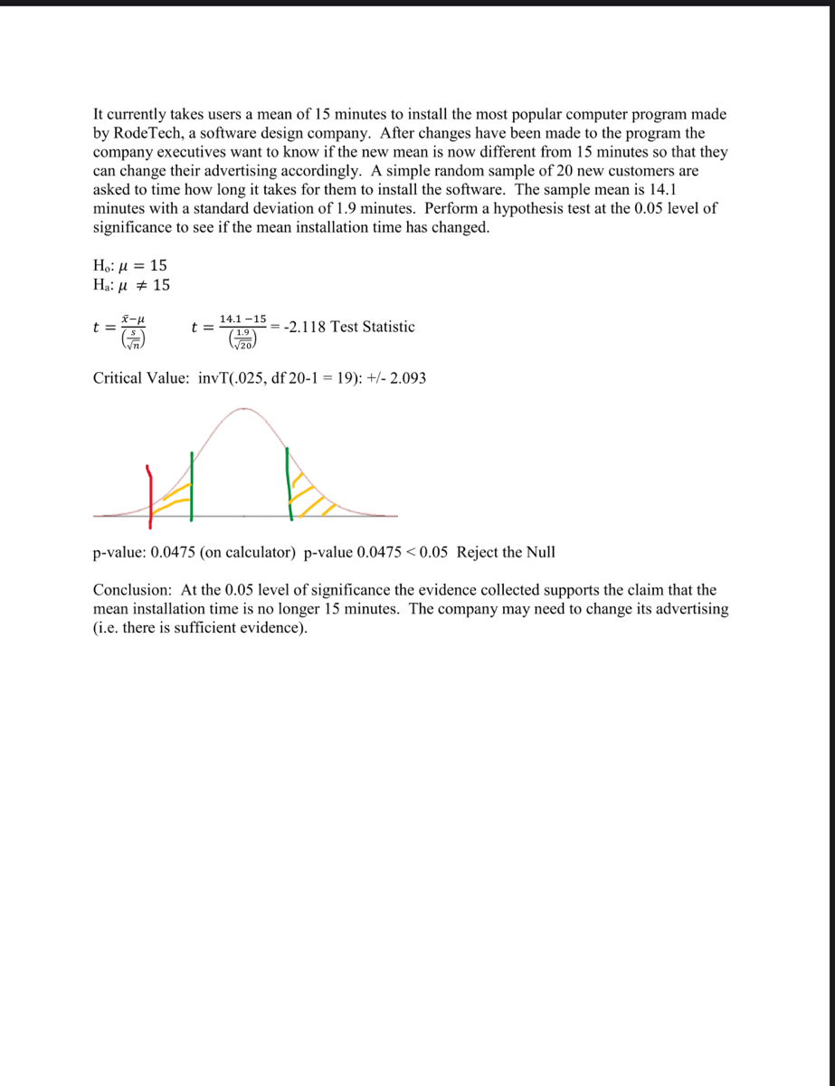
It currently takes users a mean of 15 minutes to install the most popular computer program made by RodeTech, a software design company. After changes have been made to the program the company executives want to know if the new mean is now different from 15 minutes so that they can change their advertising accordingly. A simple random sample of 20 new customers are asked to time how long it takes for them to install the software. The sample mean is 14.1 minutes with a standard deviation of 1.9 minutes. Perform a hypothesis test at the 0.05 level of significance to see if the mean installation time has changed. Ho: μ = 15 15 Ha: μ t = 14.1-15 1.9 -2.118 Test Statistic Critical Value: invT(.025, df 20-1= 19): +/- 2.093 p-value: 0.0475 (on calculator) p-value 0.0475 <0.05 Reject the Null Conclusion: At the 0.05 level of significance the evidence collected supports the claim that the mean installation time is no longer 15 minutes. The company may need to change its advertising (i.e. there is sufficient evidence). Hypothesis Testing Review - Error Analysis CNN/Money reports that the mean cost of a speeding ticket, including court fees, was $150.00 in 2002. A local police department claims that this amount has increased. To test their claim, they collect data from a simple random sample of 160 drivers who have been fined for speeding in the last year, and find that they paid a mean of $154.00 per ticket. Assuming that the population standard deviation is $17.54, is there sufficient evidence to support the police department's claim at the 0.01 level of significance? Η.: με 5 150.00 Ha: 150.00 (Right-Tailed Test) t = 1-1 t = 154-150 (17.54) √160. 2.88 Test Statistic Critical Value: invT(.01, 159): 2.35 p-value: .0022 You can find this on the calculator .0020 <0.01 Reject the Null Conclusion: At the 0.01 level of significance the evidence supports the police department's claim that the mean cost of a speeding ticked has increased (i.e. there is sufficient evidence).

Multivariate analysis is a statistical principle that involves observation and analysis of more than one statistical outcome variable at a time. O True False

Hypothesis Testing Question: Is there a statistically significant difference between the proportion of citizens in the United States and Japan without underlying health conditions who have been hospitalized after a COVID-19 diagnosis? The proportion of Americans and Japanese from nationally representative samples of adult citizens from each country who have been hospitalized for one or more days due to COVID-10 infection is reported below. Please include all steps of the five step model and write a sentence or two interpreting your results (use p= .01, Z(critical) =  ± 2.58).                          Americans                                          Japanese                         Ps1 = .07                                           Ps2 = .04                         N1 =  1325                                             N2 = 1287

Seating at GC Thinking back again to the m111survey data frame, recall that the variable seat records where each subject prefers to sit in a classroom: Front, Middle, or Back. Here is a table of the results: gcSeat <- xtabs(~seat,data=m111survey)gcSeat ## seat##  1_front 2_middle   3_back##       27       32       12 Now at Georgetown most classrooms are fairly small, with at about four rows actually in use: the first row is obviously the Front; most people would think of the second and third rows as the Middle; the fourth row would count as the Back. If preferences for the four rows are exactly the same out there in the GC population, then one would expect that: 25% of the population prefers the Front; 50% prefer the middle (twice as many rows in the Middle, after all); 25% prefer the back. We wonder if the available data provide strong evidence against the idea of equal preference among all four rows.   The results of the chi-sqaure test are as follows: ## Chi-squared test for…

Making a Decision If your claim is in the null hypothesis and you fail to reject the null hypothesis, then your conclusion would be: There is sufficient evidence to warrant rejection of the original claim There is not sufficient sample evidence to support the original claim There is not sufficient evidence to warrant rejection of the original claim The sample data support the original claim

$ 4 1.22 Stressed out, Part I. A study that surveyed a random sample of otherwise healthy high school students found that they are more likely to get muscle cramps when they are stressed. The study also noted that students drink more coffee and sleep less when they are stressed. (a) What type of study is this? (b) Can this study be used to conclude a causal relationship between increased stress and muscle cramps? (c) State possible confounding variables that might explain the observed relationship between increased stress and muscle cramps. 000 600 F4 % 5 FS A 6 MacBook Air F6 tv & 7 C F7 ▶11 * 8 S F8 AG ( 9 F9 0 F10

3-7 Hypothesis Test Business Nonathlete vs. National Av Business Athlete vs. National Average Proportion Sample Size (n) =count(range) 0 Response of Interest (ROI) Cheated Proportion Sample Size (n) =count(range) Response of Interest (ROI) Cheated Count for Response (CFR) Sample Proportion (pbar) =CFR/n Count for Response (CFR) =COUNTIF (range, ROI)| Sample Proportion (pbar) =CFR/n

using SAS

Cross Tabulation -What percentage of households headed by bachelor’s degree recipients earn $75, 000 or more?