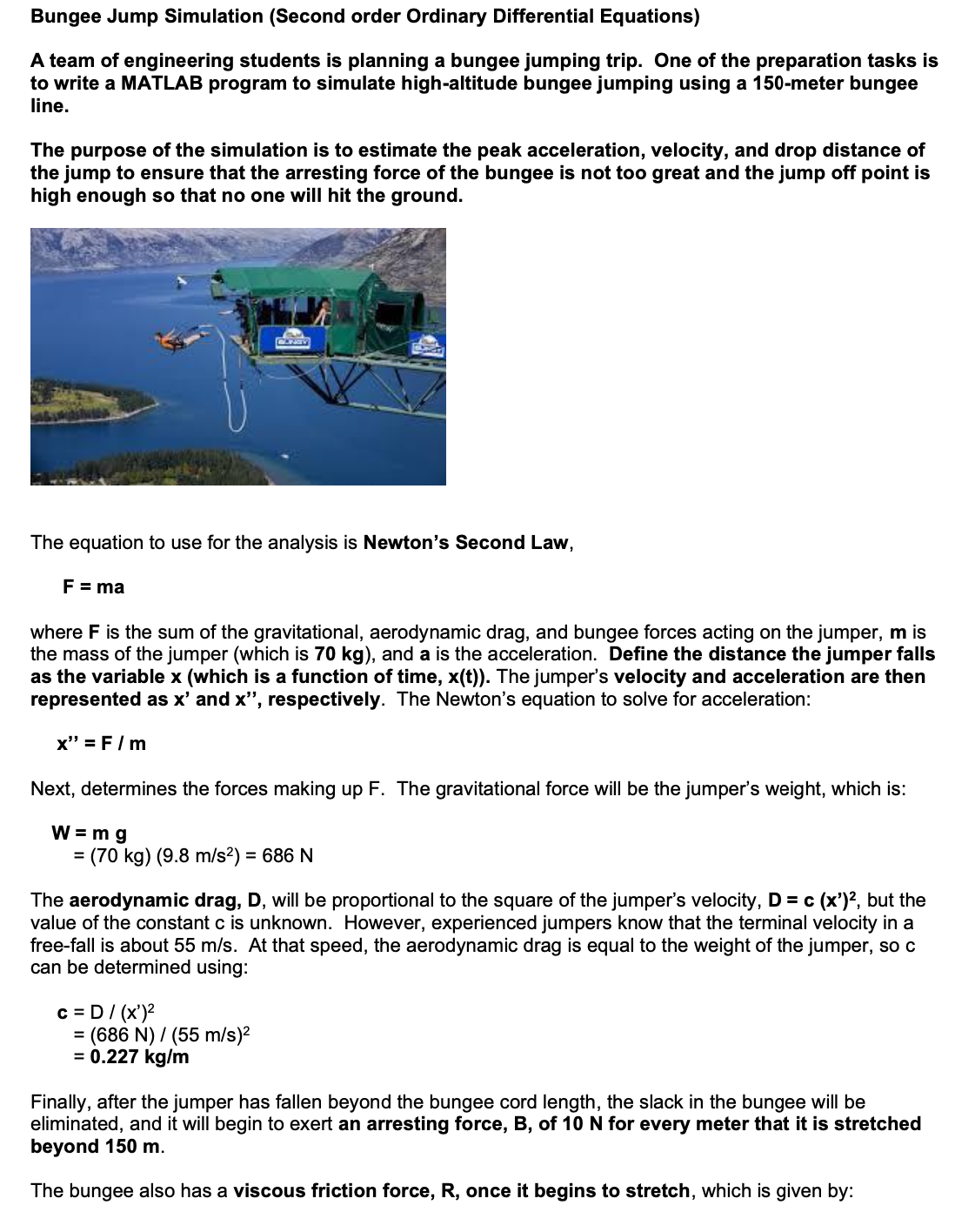
Bungee Jump Simulation (Second order Ordinary Differential Equations) A team of engineering students is planning a bungee jumping trip. One of the preparation tasks is to write a MATLAB program to simulate high-altitude bungee jumping using a 150-meter bungee line. The purpose of the simulation is to estimate the peak acceleration, velocity, and drop distance of the jump to ensure that the arresting force of the bungee is not too great and the jump off point is high enough so that no one will hit the ground. The equation to use for the analysis is Newton's Second Law, F = ma where F is the sum of the gravitational, aerodynamic drag, and bungee forces acting on the jumper, m is the mass of the jumper (which is 70 kg), and a is the acceleration. Define the distance the jumper falls as the variable x (which is a function of time, x(t)). The jumper's velocity and acceleration are then represented as x' and x", respectively. The Newton's equation to solve for acceleration: x" = F/m Next, determines the forces making up F. The gravitational force will be the jumper's weight, which is: W = mg = (70 kg) (9.8 m/s²) = 686 N The aerodynamic drag, D, will be proportional to the square of the jumper's velocity, D = c (x')², but the value of the constant c is unknown. However, experienced jumpers know that the terminal velocity in a free-fall is about 55 m/s. At that speed, the aerodynamic drag is equal to the weight of the jumper, so c can be determined using: C = D / (x')² = (686 N) (55 m/s)² = 0.227 kg/m Finally, after the jumper has fallen beyond the bungee cord length, the slack in the bungee will be eliminated, and it will begin to exert an arresting force, B, of 10 N for every meter that it is stretched beyond 150 m. The bungee also has a viscous friction force, R, once it begins to stretch, which is given by: R = -1.5 x' Thus, there will be two regions for computing the acceleration. The first equation will be used when the distance x is less than or equal to 150 m: x"=F/m = (W-D) / m = (686 -0.227 (x')²) / 70 A second equation will be used when x is greater than 150 m: x" = F/m = (W-D-B-R)/m = (686 - 0.227 (x')² - 10 (x - 150) — 1.5 x') / 70 Simulation: • • • Create one Simulink embedded function model to simulate the bungee jumper's distance (x) vs. t, the velocity (✗') vs. t and acceleration (x") vs. t for the first 500 seconds of the jump. Adjust the Simulink model maximum step size to ensure the simulation calculates enough points to obtain the maximum and minimum values of the simulation. Use the "To File" blocks in the Simulink model to save the simulation result, distance (x) vs. t, the velocity (x') vs. t and acceleration (x") vs. t, to a .mat file. Create a MATLAB program that will automatically activate the Simulink model and run the Simulink model. Load the .mat file generated by the Simulink to the MATLAB program. Use the ode45 method to simulate the bungee jumper's distance (x) vs. t, the velocity (x') vs. t and acceleration (x") vs. t for the first 500 seconds of the jump again. Generate one figure that contains 3x2 subplots to plot and compare the Simulink solution and the ode45 solution side-by-side. The figure should include the following: о ○ Plot the bungee jumper's distance (x) vs. t chart with the Simulink Solution on the left and plot the x vs. t chart using the ode45 solution on the right. Plot the bungee jumper's velocity (x') vs. t chart with the Simulink Solution on the left and plot the x' vs. t chart using the ode45 solution on the right. о Plot the bungee jumper's acceleration (x") vs. t chart with the Simulink Solution on the left and plot the x" vs. t chart using the ode45 solution on the right. Title and label plots clearly. Answer the following simulation analyses questions and print answers on screen or to a text file. • о What is the estimated peak acceleration value of the entire jump? 000 What is the estimated peak velocity of the jump? What is the estimated maximum drop distance of the jump? (How far will the jumper fall before he starts backup?) The bungee jump simulation starts at 0 seconds. How many seconds will the jumper fall to reach the maximum drop distance? From the simulation results, determine the velocity and the time when x = 150. This is the point at which the slack in the bungee is eliminated. о о о How high should the lowest jump off point be to ensure a safety factor of 2?

2. This problem has to do with the motion of a car along a straight road. The mass of the car is m, its drag resistance is Cd, the rolling resistance of the tires is pr. Choose any car that you'd like to analyze and obtain its data (cite your source). Look up typical values of rolling resistance. For the MATLAB portions, explore these questions for different values of mass of the car (which would depend on the number of passengers and luggage in the car) and the rolling resistance (which would depend on the inflation pressure of the tires) (a) Determine the differential equation if the car is traveling along a flat road. (b) Determine the traction force corresponding to speed ve. (c) (MATLAB) Determine the 0-60 mph time and distance. (d) (MATLAB) Determine the velocity and distance as a function of time if the car is to be started from rest and is supplied with the tractive force for 30 mph. (e) (MATLAB) If the car is travelling at a steady speed 30 mph and it's to be sped up to 60…

I want to run the SGP4 propagator for the ISS (ID = 25544) I got from spacetrack.org in MATLAB. I don't know where to get the inputs of the function. Where do I get the inFile and outFile that is mentioned in the following function. % Purpose: % This program shows how a Matlab program can call the Astrodynamic Standard libraries to propagate % satellites to the requested time using SGP4 method. % % The program reads in user's input and output files. The program generates an % ephemeris of position and velocity for each satellite read in. In addition, the program % also generates other sets of orbital elements such as osculating Keplerian elements, % mean Keplerian elements, latitude/longitude/height/pos, and nodal period/apogee/perigee/pos. % Totally, the program prints results to five different output files. % % % Usage: Sgp4Prop(inFile, outFile) % inFile : File contains TLEs and 6P-Card (which controls start, stop times and step size) % outFile : Base name for five output files   %…

You are part of a car accident investigative team, looking into a case where a car drove off a bridge. You are using the lab projectile launcher to simulate the accident and to test your mathematical model (an equation that applies to the situation) before you apply the model to the accident data. We are assuming we can treat the car as a projectile.

Please help me Matlab

How do I input this code for this MATLAB problem? Thanks!

I need help with a MATLAB code. I am trying to solve this question. Based on the Mars powered landing scenariosolve Eq. (14) via convex programming. Report the consumed fuel, and discuss the results with relevant plots. I am using the following MATLAB code and getting an error. I tried to fix the error and I get another one saying something about log and exp not being convex. Can you help fix my code and make sure it works.   The error is CVX Warning:  Models involving "log" or other functions in the log, exp, and entropy  family are solved using an experimental successive approximation method.  This method is slower and less reliable than the method CVX employs for  other models. Please see the section of the user's guide entitled      The successive approximation method  for more details about the approach, and for instructions on how to  suppress this warning message in the future.Error using  .*  (line 173)Disciplined convex programming error:   Cannot perform the operation:…

Don't Use Chat GPT Will Upvote And Give Handwritten Solution Please

I could really use some assistance on part b,c,d,e,f

Please show all work for c,& d as I cannot solve it for the life of myself A high-altitude skydiver of mass 100kg jumps from an altitude of 25km. Assume a near-standardatmosphere, with the following properties: d) Produce computer-generated plots of the following four quantities experienced by the sky-diver: altitude, temperature, speed, and temperature rate of change (dT /dt|skydiver). Puttime on the horizontal axis for all plots.    Use code if possible, I really need help on this, so the sooner I can be leant a hand the better