What is an Appropriate Measure of Risk?
Many attributes might be related to an asset's risk, including market capitalization (size), dividend yield, growth, price-earnings ratio, etc. The use of these traditional descriptors, however, presents a few problems:
- Most are based on accounting data which varies from firm to firm.
- Even if all firms used the same accounting rules, reporting dates differ, so constructing time-synchronized inter-firm comparisons is difficult.
- No rigorous theory tells us how traditional accounting variables should be related to an appropriate measure of risk for computing the risk-return trade-off.
Even if historical empirical relationships can be uncovered without the foundation of a rigorous theory, historical correlation might be spurious & subject to change. Currently, only two theories provide a rigorous foundation for computing trade-offs between risk & return: i.e., the Capital asset pricing model (CAPM) and Arbitrage pricing theory (APT).
Financial models incorporate macroeconomic, fundamental, and statistical factors to determine the market equilibrium and calculate the required Rate of return. There is an underlying linear relationship between the factors of the universe and the assets.
Types of Factor Model
- Single Factor
- Multi-Factor
Single-Factor Model
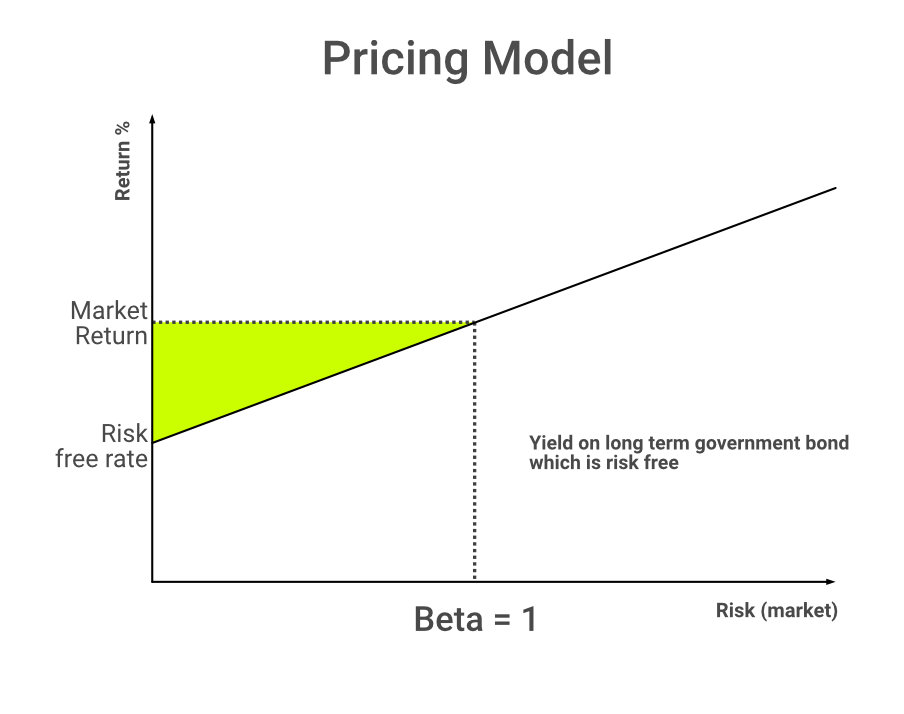
Analogy: The most common application of the Single Factor model is the Capital Asset Pricing Model (CAPM), which forms the basis of Modern Portfolio Theory.
CAPM describes the relationship between systematic risk and the expected return of the stocks. It calculates the required return based on risk measurement with a risk multiplier called the Beta coefficient (β). The CAPM model is commonly used in the finance industry for the calculation of the Weighted Average Cost of Capital/ Cost of equity.
It is based on some unreasonable assumptions such as 'the riskier the investment, the higher the return,' which might not be necessarily true in all scenarios.
Formula:
E(R)i: The expected return of Investment
Rf: Risk-Free Rate of Return
β: Beta of Investment representing volatility of Investment compared to the overall Market
E(Rm): The expected return of the Market.
E(Rm)- Rf: Market Risk Premium.
Example:
Beta(β) of a particular stock is 2 ; Market return(E(Rm) ) is 8%, Risk-free rate(Rf) is 4%.
Expected Return E(R)i= 12%
Multi-Factor Model
MFM is a financial modeling strategy where multiple factors are used to analyze asset prices. This model reveals which factors have the most impact on the price of an asset. Multi-factor portfolios can be constructed using methods like intersectional, combinational, and sequential modeling. They are commonly used by asset managers to make investment decisions and assess risk associated with investments.
Types of Multi-Factor Models
| Macroeconomic |
| Here, factors are associated with surprises in macroeconomic variables that help explain returns of asset classes. The incremental return can be calculated as the actual value less the forecasted value, and the mean of the return is typically zero. Few macroeconomic factors include: Confidence Risk: Unanticipated changes in investors' willingness to undertake relatively risky investments Time Horizon Risk: Unanticipated changes in investors' desired time to payouts Inflation Risk: Combination of Unexpected components of short- and long-run inflation rates Business Cycle Risk: Unanticipated changes in the level of real business activity |
| Fundamental |
| Here, the factors are characteristics of stocks that can be used to explain the changes in stock prices. E.g., price to earnings ratio, market capitalization & financial leverage. Fundamental factor models use asset returns, and after determining the factor sensitivities, the returns are calculated by running regressions. |
| Statistical |
| Statistical methods are applied to historical data of returns and are used to explain covariance in data. |
Construction of Multi-Factor (Three, Four, Five) Models
- Fama-French Three-Factor Model: It builds upon the Capital Asset Pricing Model, which focuses solely on the Market sensitivity, Value, and Size.
Formula:
Rs,t: Return of security s at Time t
Rf: Risk-Free Rate of Return
α: Alpha of the security, constant term of the factor model. It represents the excess return of the Investment relative to the return of the benchmark index. Higher the alpha, the better it is for investors.
F1,t, F2,t, F3,t: Macroeconomic factors like exchange rate, Inflation rate, Foreign Institutional Investors, GDP, etc.
β1, β2, β3: The factor loadings, also known as component loadings, are coefficients of the factors mentioned above.
Ě represents the error term – The equation contains an error term that is used to give further precision to the calculation. It can sometimes be used to define the security-specific news that becomes available to the investors.
Example:
| Factor | Factor sensitivity (β) | Risk Premium(F1,t) |
| Factor 1 | 0.60 (β1) | 0.05 |
| Factor 2 | 0.54 (β2) | 0.08 |
| Risk-free Rate of return (Rf ): 4% | ||
Return of security
2. Chart Four – Factor Model: It is an extra factor addition, i.e., Momentum to the Fama-French Three-Factor Model. The concept of the Momentum of an asset can be used to predict future asset returns. It uses risk-based, as well as behavioral-based, explanations to determine returns.
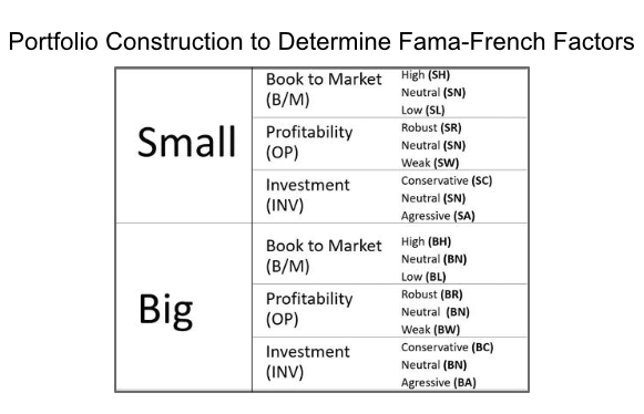
3. Fama – French Five-Factor Model: It also builds on the Three-Factor Model with two additional factors, i.e., Profitability and Investment. This model states that the value of a stock today is dependent upon future dividends. The purpose of the regression test is to observe whether the five-factor model captures average returns on the variables and to see which variables are positively or negatively correlated to each other.
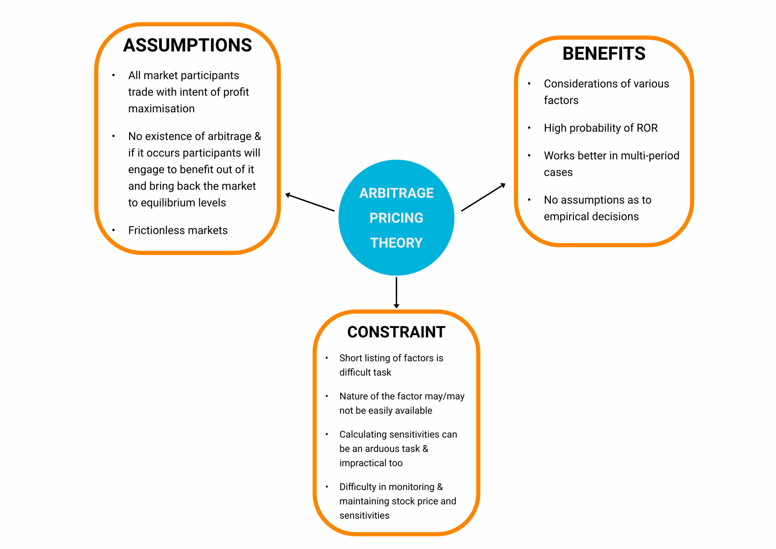
Arbitrage Pricing Theory (APT)
Analogy: Arbitrage pricing theory (APT) is a multi-factor model which says that an asset's returns can be predicted using the linear relationship between the asset's expected return and some macroeconomic variables that capture systematic risk.
Example: An insurance company is not entirely free of risk simply because it ensures a large number of individuals; natural disasters or health care changes can have an influence on insurance losses by simultaneously affecting claimants. Similarly, large, well-diversified portfolios are not risk-free because common economic forces influence all stock returns and are not eliminated by diversification. In APT, these common forces are called systematic or pervasive risks.
APT is useful to analyze portfolios from a value investing perspective to identify securities that may be temporarily mispriced. APT is based on the following assumptions:
- Asset returns are described by a linear factor model
- Asset specific risk can be eliminated by diversification as there are multiple assets
- Assets are priced in a way that no further arbitrage opportunity exists
Example:
GDP growth ßi1 = 0.6, RP1 = 4% ; Inflation rate: ßi2 = 0.8, RP2 = 2% ; Gold prices: ßi3 = -0.7, RP3 = 5% ; Standard & Poor's 500 index return: ßi4 = 1.3, RP4 = 9% ; Risk-free rate(Rf) is 3%
Common Mistakes
- Method of Selection of Factor Model
- Believing the Results without validation
- Errors in Formulas & application
- Partial Understanding of the portfolio and risk attached
Context and Applications
Factor models are mainly useful in Finance & Econometrics study; courses like CFA (Chartered Financial Analyst), portfolio management of companies, stock markets, etc.
Want more help with your economics homework?
*Response times may vary by subject and question complexity. Median response time is 34 minutes for paid subscribers and may be longer for promotional offers.
Factor Models Homework Questions from Fellow Students
Browse our recently answered Factor Models homework questions.