Concept explainers
Videos
The article “Use of Taguchi Methods and Multiple
| A | B | Hardness | |||||
| 10 | 10 | 875 | 896 | 921 | 686 | 642 | 613 |
| 10 | 25 | 712 | 719 | 698 | 621 | 632 | 645 |
| 10 | 50 | 568 | 546 | 559 | 757 | 723 | 734 |
| 20 | 10 | 876 | 835 | 868 | 812 | 796 | 772 |
| 20 | 25 | 889 | 876 | 849 | 768 | 706 | 615 |
| 20 | 50 | 756 | 732 | 723 | 681 | 723 | 712 |
| 30 | 10 | 901 | 926 | 893 | 856 | 832 | 841 |
| 30 | 25 | 789 | 801 | 776 | 845 | 827 | 831 |
| 30 | 50 | 792 | 786 | 775 | 706 | 675 | 568 |
- a. Estimate all main effects and interactions.
- b. Construct an ANOVA table. You may give
ranges for the P-values. - c. Is the additive model plausible? Provide the value of the test statistic and the P-value.
- d. Can the effect of travel speed on the hardness be described by interpreting the main effects of travel speed? If so, interpret the main effects, using multiple comparisons at the 5% level if necessary. If not, explain why not.
- e. Can the effect of accelerating voltage on the hardness be described by interpreting the main effects of accelerating voltage? If so, interpret the main effects, using multiple comparisons at the 5% level if necessary. If not, explain why not.
a.
Find all the main and interaction effects.
Answer to Problem 14E
The interaction effects are:
The main effects are:
Explanation of Solution
Calculation:
The given information is that the experiment involves the response of two factors (A (travel speed) and B (accelerating voltage)).
The first cell refers to travel speed 10 and accelerating voltage 10.
The first cell mean can be obtained as follows:
Similarly the means of remaining cells are given in the below table:
Here, the row means refers to the factor travel speed.
The first row mean can be obtained as follows:
Similarly the means of remaining rows are given in the below table:
Here, the column means refers to the factor accelerating voltage.
The first column mean can be obtained as follows:
Similarly the means of remaining columns are given in the below table:
The remaining row and column mean can be obtained as shown in the table:
| 10 | 25 | 50 | Row Mean | |
| 10 | 772.1667 | 671.1667 | 647.8333 | 697.0556 |
| 20 | 826.5 | 783.8333 | 721.1667 | 777.1667 |
| 30 | 874.8333 | 811.5 | 717 | 801.1111 |
| Column Mean | 824.5 | 755.5 | 695.3333 | 758.4444 |
The row effects can be obtained as follows:
Here,
Substitute
Substitute
Substitute
Thus, the row effects are
The column effects can be obtained as follows:
Here,
Substitute
Substitute
Substitute
Thus, the column effects are
The interaction effects can be obtained as follows:
Substitute
Substitute
Substitute
Substitute
Substitute
Substitute
Substitute
Substitute
Substitute
Thus, the interaction effects are
b.
Construct an ANOVA table and the find the ranges for the P-values.
Answer to Problem 14E
The ANOVA table is,
| Source | DF | SS | MS | F | P |
| A | 2 | 106,912 | 53,456 | 8.74 | 0.001 |
| B | 2 | 150,390 | 75,195.2 | 12.29 | 0.000 |
| Interaction | 4 | 11,409 | 2,852.2 | 0.47 | 0.760 |
| Error | 45 | 275,228 | 6,116.2 | ||
| Total | 53 | 543,939 |
For Factor A, the P-value is 0.001.
For Factor B, the P-value is 0.000.
For interaction, the P-value is 0.760.
Explanation of Solution
Calculation:
The factor A is travel speed and factor B is accelerating voltage.
Step-by-step procedure for finding the Two-Way ANOVA table is as follows:
Software procedure:
- Choose Stat > ANOVA > Two-Way.
- In Response, enter the column of Hardness.
- In Row Factor, enter the column of A.
- In Column Factor, enter the column of B.
- Click OK.
Output obtained by MINITAB procedure is as follows:
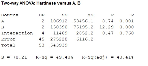
For Factor A, the F-test statistic is 8.74 and the P-value is 0.001.
For Factor B, the F-test statistic is 12.29and the P-value is 0.000.
For interaction, the F-test statistic is 0.47 and the P-value is 0.760.
c.
Explain whether the additive model is plausible.
Answer to Problem 14E
The additive model is plausible.
Explanation of Solution
Calculation:
Interaction:
Null hypothesis:
Alternative hypothesis:
For interaction, the F-test statistic is 0.47 and the P-value is 0.760.
Decision:
If
If
Conclusion:
Interaction:
Here, the P-value is greater than the level of significance.
That is,
Therefore, the null hypothesis is not rejected.
Thus, the interaction is not significant at
Therefore all the interactions are equal to zero.
Thus, the additive model is plausible.
d.
Check whether the effects of travel speed on the hardness can be described by the main effects of travel speed. If so, interpret the main effects by multiple comparisons at the 5% level. If not explain the reason.
Answer to Problem 14E
Yes, the effects of travel speed on the hardness can be described by the main effects of travel speed.
There is sufficient evidence to conclude that the effect of a travel speed of 10 differs from those of both 20 and 30 at
Explanation of Solution
Calculation:
Factor A is travel speed.
Main effect of factor A:
Null hypothesis:
Alternative hypothesis:
For Factor A, the F-test statistic is 8.74 and P- value is 0.001.
Decision:
If
If
Conclusion:
Factor A:
Here, the P-value is less than the level of significance.
That is,
Therefore, the null hypothesis is rejected.
Thus, some of the main effects of factor A are non-zero.
Hence, it is not plausible that the main effects of travel speed on the hardness are equal to zero at
Since, the main effects of travel speed on the hardness are not all equal to zero, the effects of travel speed on the hardness can be described by the main effects of travel speed.
Thus, the effects of travel speed on the hardness can be described by the main effects of travel speed.
The main effects can be interpret using Tukey’s method.
State the hypotheses:
Null hypothesis:
Alternative hypothesis:
Decision:
By Tukey’s method for multiple comparisons,
If
If
Here
From Appendix A table A.9, the upper 5% point of the
For comparing travel speed in 10 mm/s and 20 mm/s:
The 5% critical value is,
Substitute
From part (a), the row effects are
Which is greater than 63.41.
Thus, reject the null hypothesis
Hence, for travel speed in 10 mm/s and 20 mm/s there is travel speed affect the hardness.
For comparing travel speed in 10 mm/s and 30 mm/s:
Which is greater than 63.41.
Thus, reject the null hypothesis
Hence, for travel speed in 10 mm/s and 30 mm/s there is travel speed affect the hardness.
For comparing travel speed in 20 mm/s and 30 mm/s:
Which is less than 63.41.
Thus, fail to reject the null hypothesis
Hence, for travel speed in 20 mm/s and 30 mm/s there is no travel speed affect the hardness.
Conclusion:
There is sufficient evidence to conclude that the effect of a travel speed of 10 differs from those of both 20 and 30 at
e.
Check whether the effects of accelerating voltage on the hardness can be described by the main effects of accelerating voltage. If so, interpret the main effects by multiple comparisons at the 5% level. If not explain the reason.
Answer to Problem 14E
Yes, the effects of accelerating voltage on the hardness can be described by the main effects of accelerating voltage.
There is sufficient evidence to conclude that the effect of an accelerating voltage in 10 volts differs from those of both 25 volts and 50 volts at
Explanation of Solution
Calculation:
Factor B is accelerating voltage.
Main effect of factor B:
Null hypothesis:
Alternative hypothesis:
For Factor B, the F-test statistic is 12.29 and the P-value is 0.000.
Decision:
If
If
Conclusion:
Factor B:
Here, the P-value is less than the level of significance.
That is,
Therefore, the null hypothesis is rejected.
Thus, some of the main effects of factor B are zero.
Hence, it is not plausible that the main effect of accelerating voltage on the hardness are equal to zero at
Since, the main effects of accelerating voltage on the hardness are not equal to zero, the effects of accelerating voltage on the hardness can be described by the main effects of accelerating voltage.
Thus, the effects of accelerating voltage on the hardness can be described by the main effects of accelerating voltage.
The main effects can be interpret using Tukey’s method.
State the hypotheses:
Null hypothesis:
Alternative hypothesis:
Decision:
By Tukey’s method for multiple comparisons,
If
If
Here
From Appendix A table A.9, the upper 5% point of the
For comparing accelerating in 10 volts and 25 volts:
The 5% critical value is,
Substitute
From part (a), the row effects are
Which is greater than 63.41.
Thus, reject the null hypothesis
Hence, for accelerating in 10 volts and 25 volts there is accelerating voltage affect the hardness.
For comparing accelerating in 10 volts and 50 volts:
Which is greater than 63.41.
Thus, reject the null hypothesis
Hence, for accelerating in 10 volts and 50 volts there is accelerating voltage affect the hardness.
For comparing accelerating in 25 volts and 50 volts:
Which is less than 63.41.
Thus, fail to reject the null hypothesis
Hence, for accelerating in 25 volts and 50 volts there is no accelerating voltage affect the hardness.
Conclusion:
There is sufficient evidence to conclude that the effect of an accelerating voltage in 10 volts differs from those of both 25 volts and 50 volts at
Want to see more full solutions like this?
Chapter 9 Solutions
Statistics for Engineers and Scientists (Looseleaf)
Additional Math Textbook Solutions
Elementary Statistics: Picturing the World (6th Edition)
Basic Business Statistics, Student Value Edition (13th Edition)
Introduction to Statistical Quality Control
Elementary Statistics: A Step By Step Approach
Elementary Statistics Using Excel (6th Edition)
Basic Business Statistics, Student Value Edition


- Snowpacks contain a wide spectrum of pollutants thatmay represent environmental hazards. The article“Atmospheric PAH Deposition: Deposition Velocitiesand Washout Ratios” (J. of EnvironmentalEngineering, 2002: 186–195) focused on the depositionof polyaromatic hydrocarbons. The authors proposeda multiple regression model for relating depositionover a specified time period (y, in mg/m2) to tworather complicated predictors x1 (mg-sec/m3) and x2 (mg/m2), defined in terms of PAH air concentrations forvarious species, total time, and total amount of precipitation.Here is data on the species fluoranthene andcorresponding Minitab output:obs x1 x2 flth1 92017 .0026900 278.782 51830 .0030000 124.533 17236 .0000196 22.654 15776 .0000360 28.685 33462 .0004960 32.666 243500 .0038900 604.707 67793 .0011200 27.698 23471 .0006400 14.189 13948 .0004850 20.6410 8824 .0003660 20.6011 7699 .0002290 16.6112 15791 .0014100 15.0813 10239 .0004100 18.0514 43835 .0000960 99.7115 49793 .0000896 58.9716 40656…arrow_forwardWrinkle recovery angle and tensile strength are the two most important characteristics for evaluating the performance of crosslinked cotton fabric. An increase in the degree of crosslinking, as determined by ester carboxyl band absorbance, improves the wrinkle resistance of the fabric (at the expense of reducing mechanical strength). The accompanying data on x = absorbance and y = wrinkle resistance angle was read from a graph in the paper "Predicting the Performance of Durable Press Finished Cotton Fabric with Infrared Spectroscopy".t x 0.115 0.126 0.183 0.246 0.282 0.344 0.355 0.452 0.491 0.554 0.651 y 334 342 355 363 365 372 381 400 392 412 420 Here is regression output from Minitab: Predictor Constant absorb S = 3.60498 Coef 321.878 156.711 SOURCE Regression Residual Error Total R-Sq= 98.5% DF SE Coef 2.483 6.464 1 9 10 SS 7639.0 117.0 7756..0 T 129.64 24.24 P 0.000 0.000. R-Sq (adj) 98.3% MS 7639.0 13.0 F 587.81 (a) Does the simple linear regression model appear to be appropriate?…arrow_forwardThe accompanying data resulted from an experiment in which weld diameter and shear strength (in pounds) were determined for five different spot welds on steel. Below are the data collected and the regression equation. Diameter Strength 200.1 813.7 210.1 785.3 220.1 960.4 230.1 1118.0 240.0 1076.2 Strength = -941.6992 + 8.5988*Diameter a)The predicted y-hat value for a diameter of 201 is 864. Interpret this predicted value. b)what is the predicted strength of a weld with a diameter of 51?arrow_forward
- Which non-parametric test for ordinal data is the best to use in the given scenario? In a study by Zuckerman and Heneghan, hemodynamic stresses were measured on subjects undergoing laparoscopic cholecystectomy. An outcome variable of interest was the ventricular end-diastolic volume (LVEDV) measured in mm. A portion of the data appears in the following table. Baseline refers to a measurement taken 5 minutes after induction of anesthesia, and the term '5 minutes' refers to a measurement taken 5 minutes after baseline. Can we conclude that, on the basis of these data, among subjects undergoing laparoscopic cholecystectomy, the average LVEDV levels change? Let a =.01. LVEDV (ml) Subject Baseline 5 minutes 1 51.7 49.3 2 79.0 72.0 3 78.7 67.0 4 80.3 70.4 5 72.0 65.9 6 85.0 84.8 7 79.0 77.7 8 71.3 74.0 9 54.3 58.0 10 58.8 65.0 a. Mood Median Test b. Sign Test c. Wilcoxon Rank Sum Test d. Wilcoxon Matched-Pair Signed-Ranks Test e. Spearman and Kendall Correlation…arrow_forward3. Wine Participant magazine has collected average price per bottle for the prestigious Chateau Le Thundebird bordeaux for different vintages (years). The data appears in the table below. year of bottling price a) draw the scatter diagram showing how wine price varies by vintage year b) use the most appropriate regression equation to determine the relationship between year of bottling (age) and price. c) what is the explanatory power (RSQ) of that equation d) determine the predicted price of a bottle of this wine for the 2017 vintage. 2009 36 2010 40 2011 51 2012 60 2013 68 2014 72 2015 70 2016 65 2018 51 2019 44 2020 39arrow_forwardFoot ulcers are a common problem for people with diabetes. Higher skin temperatures on the foot indicate an increased risk of ulcers. The article "An Intelligent Insole for Diabetic Patients with the Loss of Protective Sensation" (Kimberly Anderson, M.S. Thesis, Colorado School of Mines), reports measurements of temperatures, in °F, of both feet for 181 diabetic patients. The results are presented in the following table. Left Foot Right Foot 80 80 85 85 75 80 88 86 89 87 87 82 78 78 88 89 89 90 76 81 89 86 87 82 78 78 80 81 87 82 86 85 76 80 88 89 Construct a scatterplot of the right foot temperature (y) versus the left foot temperature (x). Verify that a linear model is appropriate. b. Compute the least-squares line for predicting the right foot temperature from the left foot temperature. If the left foot temperatures of two patients differ by 2 degrees, by how much would you predict their right foot temperatures to differ? Predict the right foot temperature for a patient whose left…arrow_forward
- The article "Influence of Freezing Temperature on Hydraulic Conductivity of Silty Clay" (J. Konrad and M. Samson, Journal of Geotechnical and Geoenvironmental Engineering, 2000:180–187) describes a study of factors affecting hydraulic conductivity of soils. The measurements of hydraulic conductivity in units of 108 cm/s (y), initial void ratio (x), and thawed void ratio (x2) for 12 specimens of silty clay are presented in the following table. y 1.01 1.12 1.04 1.30 1.01 1.04 0.955 1.15 1.23 1.28 1.23 1.30 0.84 0.88 0.85 0.95 0.88 0.86 0.85 0.89 0.90 0.94 0.88 0.90 X1 0.81 0.85 0.87 0.92 0.84 0.85 0.85 0.86 0.85 0.92 0.88 0.92 X2 Fit the model y = Bo + fix1 + e. For each coefficient, test the null hypothesis that it is equal to 0. Fit the model y = Bo + Bzx2 + e. For each coefficient, test the null hypothesis that it is equal to 0. Fit the model y = Bo + BzX1 + Bzxz + e. For each coefficient, test the null hypothesis that it is equal to 0. d. Which of the models in parts (a) to (c) is…arrow_forwardWhich of the non-parametric test for ordinal data is the best to use in the given scenario? An experiment was conducted to compare the strengths of two types of elastic bandages: one a standard bandage of a specified weight and the other the same standard but treated with a chemical substance. Ten pieces of each were randomly selected from production. Does the treated bandage tend to be stronger than the standard? Table 1. Strength measurements (and their ranks) for 2 types of bandages. STANDARD TREATED 1.21(2) 1.49(15) 1.43(12) 1.37(7.5) 1.35(6) 1.67(20) 1.51(17) 1.50(16) 1.39(9) 1.31(5) 1.17(1) 1.29(3.5) 1.48(14) 1.52(18) 1.42(11) 1.37(7.5) 1.29(3.5) 1.44(13) 1.4(10) 1.53(19) a. Mood median test b. sign test c. Wilcoxon rank-sum test d. Wilcoxon matched-pairs signed-ranks test e. Spearman and Kendall correlation coefficients f. Kruskal-Wallis testarrow_forwardThe article "Modeling Resilient Modulus and Temperature Correction for Saudi Roads" (H. Wahhab, I. Asi, and R. Ramadhan, Journal of Materials in Civil Engineering, 2001:298– 305) describes a study designed to predict the resilient modulus of pavement from physical properties. The following table presents data for the resilient modulus at 40°Cin10® kPa (y), the surface area of the aggregate in m²/kg (x1), and the softening point of the asphalt in °C (х). y X1 X2 1.48 5.77 60.5 1.70 7.45 74.2 2.03 8.14 67.6 2.86 8.73 70.0 2.43 7.12 64.6 3.06 6.89 65.3 2.44 8.64 66.2 1.29 6.58 64.1 3.53 9.10 68.6 1.04 8.06 58.8 1.88 5.93 63.2 1.90 8.17 62.1 1.76 9.84 68.9 2.82 7.17 72.2 1.00 7.78 54.1 The full quadratic model is y = + P,x, + PzX, + Pz*jXz + Pxx¡ + Bzx; + €. Which submodel of this full model do you believe is most appropriate? Justify your answer by fitting two or more models and comparing the results.arrow_forward
- Aa Febru The body mass index (BMI) of a person is defined to be the person's body mass divided by the square of the person's height. The article "Influences of Parameter Uncertainties within the ICRP 66 Respiratory Tract Model: Particle Deposition" (W. Bolch, E. Farfan, et al., Health Physics, 2001:378-394) states that body mass index (in kg/m2) in men aged 25-34 is lognormally distributed with parameters u = 3.215 and o = 0.157. a.Find the mean and standard deviation BMI for men aged 25-34. b.Find the standard deviation of BMI for men aged 25-34. c.Find the median BMI for men aged 25-34. d.What proportion of men aged 25-34 have a BMI less than 20? e.Find the 80th percentile of BMI for men agėd 25 -34. 04... Rext 田arrow_forward1. Analyze the data as a two way factorial design. Johnson and Leone (Statistics and Experimental Design in Engineering and the Physical Sciences, Wiley, 977) describe an experiment to investigate warping of copper plates. The two factors studied were the temperature and the copper content of the plates. The response variable was a measure of the amount of warping. The data were as follows: Temperature (°C) 50 75 100 125 40 17, 20 12,9 16, 12 21, 17 Copper Content (%) 60 80 16, 21 18, 13 18, 21 23, 2! 24, 22 17, 12 25, 23 23, 22 100 28, 27 27, 31 30, 23 29, 31arrow_forwarda) We conduct a regression of size on hhinc, owner, hhsize, hhsize2,and hhsize3. We do not include the constant. The regression output is reported in Table 3. Would you conclude that the home size increases with the household size? Interpret the sign and magnitude of the estimated coefficients of hhsize1, hhsize2, and hhsize3.arrow_forward
 MATLAB: An Introduction with ApplicationsStatisticsISBN:9781119256830Author:Amos GilatPublisher:John Wiley & Sons Inc
 Probability and Statistics for Engineering and th...StatisticsISBN:9781305251809Author:Jay L. DevorePublisher:Cengage Learning
 Statistics for The Behavioral Sciences (MindTap C...StatisticsISBN:9781305504912Author:Frederick J Gravetter, Larry B. WallnauPublisher:Cengage Learning
 Elementary Statistics: Picturing the World (7th E...StatisticsISBN:9780134683416Author:Ron Larson, Betsy FarberPublisher:PEARSON
 The Basic Practice of StatisticsStatisticsISBN:9781319042578Author:David S. Moore, William I. Notz, Michael A. FlignerPublisher:W. H. Freeman
 Introduction to the Practice of StatisticsStatisticsISBN:9781319013387Author:David S. Moore, George P. McCabe, Bruce A. CraigPublisher:W. H. Freeman