In Problems 8-12, please use the following steps (i)-(v) for all hypothesis tests: (i) What is the level of significance? State the null and alternate hypotheses. (ii) Check Requirements What sampling distribution will you use? What assumptions are you making? What is the value of the sample test statistic? (iii) Find (or estimate) the P -value. Sketch the sampling distribution and show the area corresponding to the P -value. (iv) Based on your answers in parts (i)-(iii), will you reject or fail to reject the null hypothesis? Are the data statistically significant at level a? (v) Interpret your conclusion in the context of the application. Note: For degrees of freedom d.f. not in the Student’s t table, use the closet d.f. that is smaller . In some situation, this choice of d.f. may increase the P -value a small amount and thereby produce a slightly more "conservative” answer. Testing and Estimating µ with σ Unknown Carboxyhemoglobin is formed when hemoglobin is exposed to carbon monoxide. Heavy smokers tend to have a high percentage of carboxyhemoglobin in their blood (Reference: A Manual of Laboratory and Diagnostic Tests by F. Fischbach). Let x be a random variable representing percentage of carboxyhemoglobin in the blood. For a person who is a regular heavy smoker, x has a distribution that is approximately normal. A random sample of n = 12 blood tests given to a heavy smoker gave the following results (percentage of carboxyhemoglobin in the blood): 9.1 9.5 10.2 9.8 11.3 12.2 11.6 10.3 8.9 9.7 13.4 9.9 (a) Use a calculator to verify that x ¯ ≈ 10.49 and s ≈ 1.36 . (b) A long-term population mean µ = 10% is considered a health risk. However, a long-term population mean above 10% is considered a clinical alert that the person may be asymptomatic. Do the data indicate that the population mean percentage is higher than 10% for this patient? Use α = 0.05. (c) Use the given data to find a 99% confidence interval for µ for this patient.

Question

Want to see more full solutions like this?

Answer 1

Textbook Question

Chapter 9, Problem 9CRP

In Problems 8-12, please use the following steps (i)-(v) for all hypothesis tests:

(i) What is the level of significance? State the null and alternate hypotheses.

(ii) Check Requirements What sampling distribution will you use? What assumptions are you making? What is the value of the sample test statistic?

(iii) Find (or estimate) the P-value. Sketch the sampling distribution and show the area corresponding to the P-value.

(iv) Based on your answers in parts (i)-(iii), will you reject or fail to reject the null hypothesis? Are the data statistically significant at level a?

(v) Interpret your conclusion in the context of the application.

Note: For degrees of freedom d.f. not in the Student’s t table, use the closet d.f. that is smaller. In some situation, this choice of d.f. may increase the P-value a small amount and thereby produce a slightly more "conservative” answer.

Testing and Estimating µ with σ Unknown Carboxyhemoglobin is formed when hemoglobin is exposed to carbon monoxide. Heavy smokers tend to have a high percentage of carboxyhemoglobin in their blood (Reference: A Manual of Laboratory and Diagnostic Tests by F. Fischbach). Let x be a random variable representing percentage of carboxyhemoglobin in the blood. For a person who is a regular heavy smoker, x has a distribution that is approximately normal. A random sample of n = 12 blood tests given to a heavy smoker gave the following results (percentage of carboxyhemoglobin in the blood):

9.1	9.5	10.2	9.8	11.3	12.2
11.6	10.3	8.9	9.7	13.4	9.9

(a) Use a calculator to verify that $x ¯ ≈ 10.49$ and $s ≈ 1.36$ .

(b) A long-term population mean µ = 10% is considered a health risk. However, a long-term population mean above 10% is considered a clinical alert that the person may be asymptomatic. Do the data indicate that the population mean percentage is higher than 10% for this patient? Use α = 0.05.

(c) Use the given data to find a 99% confidence interval for µ for this patient.

(a)

Expert Solution

To determine

Whether the sample mean $x¯=10.49$ and sample standard deviation $s=1.36$ .

Answer to Problem 9CRP

Solution:

Yes, the sample mean $x¯=10.49$ and sample standard deviation $s=1.36$ .

Explanation of Solution

To calculate the required statistics using the Minitab, follow the below instructions:

Step 1: Go to the Minitab software.

Step 2: Go to Stat >Basic statistics > Display Descriptive Statistics.

Step 3: Select ‘Percentages’ in variables.

Step 4: Click on OK.

The obtained statistics is:

Descriptive Statistics: Percentages

Statistics

Variable	N	N*	Mean	SE Mean	StDev	Minimum	Q1	Median	Q3	Maximum
Percentages	12	0	10.492	0.392	1.358	8.900	9.550	10.050	11.525	13.400

From the Minitab output, the sample mean and sample standard deviation are approximately equals to $x¯=10.49$ and $s=1.36$ .

(b)

(i)

Expert Solution

To determine

The level of significance, null and alternative hypothesis.

Answer to Problem 9CRP

Solution:

The level of significance is $α=0.05$ . The null hypothesis is $H0:μ=10$ and alternative hypothesis $H1:μ>10$ .

Explanation of Solution

The level of significance is defined as the probability of rejecting the null hypothesis when it is true, it is denoted by $α=0.05$ .

Null hypothesis $H0:μ=10$

Alternative hypothesis $H1:μ>10$

(ii)

Expert Solution

To determine

To find:

The sampling distribution that should be used and compute the value of the sample test statistic.

Answer to Problem 9CRP

Solution:

The student's t distribution should be used. The sample test statisticis 1.25.

Explanation of Solution

Calculation:

We assume that x distribution is mound shape and symmetrical, because $σ$ is unknown, we can use student's t distribution with $d.f=n−1=11$ .

Using $x¯=10.49, μ=10, s=1.36, n=12$

The sample test statistic t is

$t=(x¯−μ)snt=(10.49−10)1.3612t=1.25$

(iii)

Expert Solution

To determine

To find:

The P-value of the test statistic and sketch the sampling distribution showing the area corresponding to the P-value.

Answer to Problem 9CRP

Solution:

The P-value of the test statistic is 0.1186.

Explanation of Solution

Calculation:

We have t = 1.25

$P−value = P(t>1.25) =1−P(t<1.25)$

Using Table 4 from the Appendix to find the specified area:

$0.10<P−value <0.125$

Graph:

To draw the required graphs using the Minitab, follow the below instructions:

Step 1: Go to the Minitab software.

Step 2: Go to Graph > Probability distribution plot > View probability.

Step 3: Select ‘t’ and enter d.f = 11.

Step 4: Click on the Shaded area > X value.

Step 5: Enter X-value as 1.25 and select ‘Right Tail’.

Step 6: Click on OK.

The obtained distribution graph is:

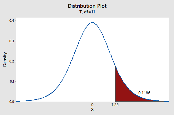
Understanding Basic Statistics, Chapter 9, Problem 9CRP

$P−value = 0.1186$

(iv)

Expert Solution

To determine

Whether we reject or fail to reject the null hypothesisand whether the data is statistically significant for a level of significance of 0.05.

Answer to Problem 9CRP

Solution:

The P-value $>α$ , hence we failed to reject the $H0$ . The data is not statistically significant for a level of significance of 0.05.

Explanation of Solution

The P-value of 0.1186 is greater than the level of significance (α) of 0.05. Therefore we failed to reject the null hypothesis $H0$ . Hence, the data is not statistically significant for a level of significance of 0.05.

(v)

Expert Solution

To determine

The interpretation for the conclusion.

Answer to Problem 9CRP

Solution:

There is not enough evidence to conclude that sample mean of 12 smokers' Carboxyhoemoglobin levels is significantly large enough to sound a clinical alert.

Explanation of Solution

The P-value is greater than the level of significance ( $α$ ) of 0.05. Therefore we failed to reject the null hypothesis $H0$ . There is not enough evidence to conclude that sample mean of 12 smokers' Carboxyhoemoglobin levels is significantly large enough to sound a clinical alert.

(b)

Expert Solution

To determine

To find:

A 99% confidence interval for the mean for this patient.

Answer to Problem 9CRP

Solution:

The 99% confidence interval for $μ$ is (9.27, 11.71).

Explanation of Solution

Calculation:

We have to find 99% confidence interval

$c=0.99 and d.f.=11Using Table 4 of Appendixt0.99=3.106s=1.36n=12E=tcsnE=3.1061.3612E=1.2194E≈1.22$

Then, the 99% confidence interval is

$x¯−E<μ<x¯+E10.49−1.22<μ<10.49+1.229.27<μ<11.71$

The 99% confidence interval for $μ$ is (9.27, 11.71).

Want to see more full solutions like this?

Subscribe now to access step-by-step solutions to millions of textbook problems written by subject matter experts!

Students have asked these similar questions

Business discuss

Analyze the residuals of a linear regression model and select the best response. yes, the residual plot does not show a curve no, the residual plot shows a curve yes, the residual plot shows a curve no, the residual plot does not show a curve I answered, "No, the residual plot shows a curve." (and this was incorrect). I am not sure why I keep getting these wrong when the answer seems obvious. Please help me understand what the yes and no references in the answer.

a. Find the value of A.b. Find pX(x) and py(y).c. Find pX|y(x|y) and py|X(y|x)d. Are x and y independent? Why or why not?

Answer 2