Statistical Reasoning for Everyday Life (5th Edition)
5th Edition
ISBN: 9780134494043
Author: Jeff Bennett, William L. Briggs, Mario F. Triola
Publisher: PEARSON
expand_more
expand_more
format_list_bulleted
Concept explainers
Videos
Textbook Question
Chapter 6.4, Problem 11E
Commercial Aviation. For Exercises 9–12, use the following table, which summarizes some data on commercial aviation flights in the United States for three separate years.
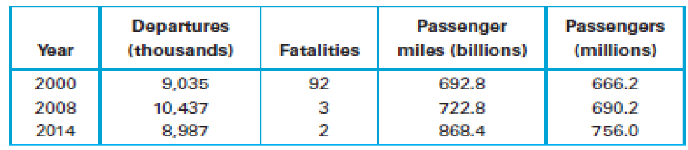
- 11. For each of the three years, find the fatality rate in deaths per million passengers. On the basis of those rates, which year was the safest? Why?
Expert Solution & Answer
Want to see the full answer?
Check out a sample textbook solution
Students have asked these similar questions
please solve parts d e f
2.62 For the period 2001–2008, the Bristol-Myers Squibb Company, Inc. reported the following amounts (in billions of dollars) for (1) net sales and (2) advertising and product promotion. The data are also in the file XR02062.
Source: Bristol-Myers Squibb Company, Annual Reports, 2005, 2008.
Year Net Sales Advertising/Promotion
2001 $16.612 $1.201
2002 16.208 1.143
2003 18.653 1.416
2004 19.380 1.411
2005 19.207 1.476
2006 16.208 1.304
2007 18.193 1.415
2008 20.597 1.550
For these data, construct a line graph that shows both net sales and expenditures for advertising/product promotion over time. Some would suggest that increases in advertising should be accompanied by increases in sales. Does your line graph support this?
Because of high tuition costs at state and private universities, enrollments atcommunity colleges have increased dramatically in recent years. The following data show theenrollment (in thousands) for Jefferson Community College from 2001–2009:Year Period (t) Enrollment (1000s)2001 1 6.52002 2 8.12003 3 8.42004 4 10.22005 5 12.52006 6 13.32007 7 13.72008 8 17.22009 9 18.1Compute F10: the Forecast for 2010. Compute Pearson’s Correlation Coefficient Use the Method of Least Squares to obtain the Best-Fit-Line for this data. Use the line to compute the forecast.
Chapter 6 Solutions
Statistical Reasoning for Everyday Life (5th Edition)
Ch. 6.1 - Coin Tossing. Suppose you toss a coin 100 times....Ch. 6.1 - Statistical Significance. What do we mean when we...Ch. 6.1 - Prob. 3ECh. 6.1 - Quantifying Significance. What does it mean to say...Ch. 6.1 - Does It Make Sense? For Exercises 58, determine...Ch. 6.1 - Does It Make Sense? For Exercises 58, determine...Ch. 6.1 - Does It Make Sense? For Exercises 58, determine...Ch. 6.1 - Does It Make Sense? For Exercises 58, determine...Ch. 6.1 - Subjective Significance. For each event in...Ch. 6.1 - Subjective Significance. For each event in...
Ch. 6.1 - Subjective Significance. For each event in...Ch. 6.1 - Subjective Significance. For each event in...Ch. 6.1 - Subjective Significance. For each event in...Ch. 6.1 - Subjective Significance. For each event in...Ch. 6.1 - Subjective Significance. For each event in...Ch. 6.1 - Subjective Significance. For each event in...Ch. 6.1 - Prob. 17ECh. 6.1 - Carpal Tunnel Syndrome Treatments. An experiment...Ch. 6.1 - Prob. 19ECh. 6.1 - Prob. 20ECh. 6.1 - Human Body Temperature. In a study by researchers...Ch. 6.1 - Seat Belts and Children. In a study of children...Ch. 6.1 - Prob. 23ECh. 6.1 - Subjective Significance. For each event in...Ch. 6.2 - Outcomes and Events. Distinguish between an...Ch. 6.2 - Notation. What does it mean when we write P(A)?...Ch. 6.2 - Probability Types. Briefly describe the...Ch. 6.2 - Prob. 4ECh. 6.2 - Prob. 5ECh. 6.2 - Does It Make Sense? For Exercises 58, determine...Ch. 6.2 - Prob. 7ECh. 6.2 - Does It Make Sense? For Exercises 58, determine...Ch. 6.2 - Counting Outcomes. How many different three-child...Ch. 6.2 - Prob. 10ECh. 6.2 - Theoretical Probabilities. For Exercises 1120, use...Ch. 6.2 - Theoretical Probabilities. For Exercises 1120, use...Ch. 6.2 - Theoretical Probabilities. For Exercises 1120, use...Ch. 6.2 - Theoretical Probabilities. For Exercises 1120, use...Ch. 6.2 - Theoretical Probabilities. For Exercises 1120, use...Ch. 6.2 - Theoretical Probabilities. For Exercises 1120, use...Ch. 6.2 - Theoretical Probabilities. For Exercises 1120, use...Ch. 6.2 - Theoretical Probabilities. For Exercises 1120, use...Ch. 6.2 - Theoretical Probabilities. For Exercises 1120, use...Ch. 6.2 - Theoretical Probabilities. For Exercises 1120, use...Ch. 6.2 - Days of the Week. What is the probability of...Ch. 6.2 - Days of the Week. What is the probability of...Ch. 6.2 - Complementary Events. Exercises 2330 involve...Ch. 6.2 - Complementary Events. Exercises 2330 involve...Ch. 6.2 - Complementary Events. Exercises 2330 involve...Ch. 6.2 - Complementary Events. Exercises 2330 involve...Ch. 6.2 - Complementary Events. Exercises 2330 involve...Ch. 6.2 - Complementary Events. Exercises 2330 involve...Ch. 6.2 - Prob. 29ECh. 6.2 - Prob. 30ECh. 6.2 - Theoretical Probabilities. For Exercises 3134, use...Ch. 6.2 - Theoretical Probabilities. For Exercises 3134, use...Ch. 6.2 - Theoretical Probabilities. For Exercises 3134, use...Ch. 6.2 - Theoretical Probabilities. For Exercises 3134, use...Ch. 6.2 - Relative Frequency Probabilities. Use the relative...Ch. 6.2 - Relative Frequency Probabilities. Use the relative...Ch. 6.2 - Relative Frequency Probabilities. Use the relative...Ch. 6.2 - Prob. 38ECh. 6.2 - Probability Distributions. In Exercises 39 and 40,...Ch. 6.2 - Probability Distributions. In Exercises 39 and 40,...Ch. 6.3 - Law of Large Numbers. What is the law of large...Ch. 6.3 - Understanding the Law of Large Numbers. In terms...Ch. 6.3 - Expected Value. What is an expected value, and how...Ch. 6.3 - Gamblers Fallacy. What is the gamblers fallacy?...Ch. 6.3 - Prob. 5ECh. 6.3 - Does It Make Sense? For Exercises 58, determine...Ch. 6.3 - Prob. 7ECh. 6.3 - Does It Make Sense? For Exercises 58, determine...Ch. 6.3 - Gender Selection. In analyzing genders of...Ch. 6.3 - Speedy Driver. A person who has a habit of driving...Ch. 6.3 - Should You Play? Suppose you are offered this...Ch. 6.3 - Kentuckys Pick 4 Lottery. If you bet 1 in...Ch. 6.3 - Expected Value for Life Insurance. There is a...Ch. 6.3 - Expected Value for Life Insurance There is a...Ch. 6.3 - Expected Waiting Time. You arrive at a bus stop...Ch. 6.3 - Expected Value in Roulette. As shown in Figure...Ch. 6.3 - Expected Value in Casino Dice. When you give a...Ch. 6.3 - New Jersey Pick 4. In New Jerseys Pick 4 lottery,...Ch. 6.3 - Extra Points in Football. Football teams have the...Ch. 6.3 - Prob. 20ECh. 6.3 - Psychology of Expected Values. In 1953, a French...Ch. 6.3 - Behind in Coin Tossing: Can You Catch Up? Suppose...Ch. 6.4 - Risk and Travel. What is travel risk? Give an...Ch. 6.4 - Prob. 2ECh. 6.4 - Prob. 3ECh. 6.4 - Prob. 4ECh. 6.4 - Prob. 5ECh. 6.4 - Does It Make Sense? For Exercises 58, determine...Ch. 6.4 - Prob. 7ECh. 6.4 - Prob. 8ECh. 6.4 - Prob. 9ECh. 6.4 - Commercial Aviation. For Exercises 912, use the...Ch. 6.4 - Commercial Aviation. For Exercises 912, use the...Ch. 6.4 - Prob. 12ECh. 6.4 - Births/Deaths. For Exercises 1316, use the data in...Ch. 6.4 - Births/Deaths. For Exercises 1316, use the data in...Ch. 6.4 - Births/Deaths. For Exercises 1316, use the data in...Ch. 6.4 - Births/Deaths. For Exercises 1316, use the data in...Ch. 6.4 - Vital Statistics. For Exercises 1720, use the data...Ch. 6.4 - Vital Statistics. For Exercises 1720, use the data...Ch. 6.4 - Prob. 19ECh. 6.4 - Prob. 20ECh. 6.4 - Prob. 21ECh. 6.4 - Prob. 22ECh. 6.4 - Prob. 23ECh. 6.4 - Prob. 24ECh. 6.4 - Prob. 25ECh. 6.4 - Prob. 26ECh. 6.4 - Prob. 27ECh. 6.4 - Prob. 28ECh. 6.4 - Life in This Century. Example 5 assumed that the...Ch. 6.4 - Prob. 30ECh. 6.5 - Independence. Let A denote the event of getting a...Ch. 6.5 - Independence. A geneticist is working with 3 green...Ch. 6.5 - Prob. 3ECh. 6.5 - Complementary Events. Let A be the event of...Ch. 6.5 - Prob. 5ECh. 6.5 - Does It Make Sense? For Exercises 58, determine...Ch. 6.5 - Does It Make Sense? For Exercises 58, determine...Ch. 6.5 - Does It Make Sense? For Exercises 58, determine...Ch. 6.5 - Births. Assume that boys and girls are equally...Ch. 6.5 - Births. A couple plans to have four children. Find...Ch. 6.5 - Password. A programmer is instructed to create a...Ch. 6.5 - Wearing Hunter Orange. A study of hunting injuries...Ch. 6.5 - Songs. The 50 songs on a smartphone consist of 15...Ch. 6.5 - Polls. A pollster plans to call adults. She has a...Ch. 6.5 - Probability and Court Decisions. In Exercises...Ch. 6.5 - Probability and Court Decisions. In Exercises...Ch. 6.5 - Probability and Court Decisions. In Exercises...Ch. 6.5 - Probability and Court Decisions. In Exercises...Ch. 6.5 - Probability and Court Decisions. In Exercises...Ch. 6.5 - Probability and Court Decisions. In Exercises...Ch. 6.5 - Prob. 21ECh. 6.5 - Pedestrian Deaths. For Exercises 2126, use the...Ch. 6.5 - Prob. 23ECh. 6.5 - Pedestrian Deaths. For Exercises 2126, use the...Ch. 6.5 - Prob. 25ECh. 6.5 - Pedestrian Deaths. For Exercises 2126, use the...Ch. 6.5 - Clinical Trial. In a clinical trial of an allergy...Ch. 6.5 - Prob. 28ECh. 6.5 - Prob. 29ECh. 6.5 - Survey Refusals. Refer to the data in Exercise 29....Ch. 6.5 - Drug Testing. A 1-Panel-THC test for marijuana use...Ch. 6.5 - BINGO. The game of BINGO involves drawing numbered...Ch. 6 - For Exercises 17, use the data in the following...Ch. 6 - For Exercises 17, use the data in the following...Ch. 6 - For Exercises 17, use the data in the following...Ch. 6 - For Exercises 17, use the data in the following...Ch. 6 - For Exercises 17, use the data in the following...Ch. 6 - For Exercises 17, use the data in the following...Ch. 6 - For Exercises 17, use the data in the following...Ch. 6 - The Binary Computer Company manufactures computer...Ch. 6 - For a recent year, the fatality rate from motor...Ch. 6 - A Las Vegas handicapper can correctly predict the...Ch. 6 - For the handicapper in Exercise 1, find the...Ch. 6 - In a clinical trial of the effectiveness of a...Ch. 6 - If P(A) = 0.65, what is the value of P(not A)?Ch. 6 - In Exercises 610, use the following results. The...Ch. 6 - In Exercises 610, use the following results. The...Ch. 6 - Prob. 8CQCh. 6 - In Exercises 610, use the following results. The...Ch. 6 - In Exercises 610, use the following results. The...
Knowledge Booster


Learn more about
Need a deep-dive on the concept behind this application? Look no further. Learn more about this topic, statistics and related others by exploring similar questions and additional content below.Similar questions
- A neighborhood is trying to set up school carpools, but they need to determine the number of students who need to travel to the elementary school (ages 5–10), the middle school (ages 11–13), and the high school (ages 14–18). A histogram summarizes their findings: Histogram titled Carpool, with Number of Children on the y axis and Age Groups on the x axis. Bar 1 is 5 to 10 years old and has a value of 3. Bar 2 is 11 to 13 years old and has a value of 7. Bar 3 is 14 to 18 years old and has a value of 4. Which of the following data sets is represented in the histogram? A. {3, 3, 3, 7, 7, 7, 7, 7, 7, 7, 4, 4, 4, 4} B. {5, 10, 4, 11, 12, 13, 12, 13, 12, 11, 14, 14, 19, 18} C. {5, 6, 5, 11, 12, 13, 12, 13, 14, 15, 11, 18, 17, 13} D. {3, 5, 10, 11, 13, 7, 18, 14, 4}arrow_forwardIn Exercises 37–40, determine the value of k.arrow_forwardFor Exercises 7–10, (a) compute the arithmetic mean and (b) indicate whether it is a 7. There are 10 salespeople employed by Midtown Ford. The number of new cars statistic or a parameter. Sold last month by the respective salespeople were: 15, 23, 4, 19, 18, 10, 10, 0 28, 19. Dve order company counted the number of incoming calls per day to the compa- Ivs toll-free number during the first 7 days in May: 14, 24, 19, 31, 36, 26, 17.arrow_forward
- Use the table to answer the following questions. Year U.S population (millions) Traffic fatalities Licensed drivers(millions) Vehicle-miles (trillions) 1995 263 41,817 177 2.4 2015 321 35,092 218 3.1 Find and compare death rates per person and per 100,000 people for traffic fatalities per two years. Express the 1995 and 2015 fatality rates in deaths per100 million vehicle-miles traveled. Express the 1995 and 2015 fatality rates in deaths per 100,000 population. Express the 1995 and 2015 fatality rates in deaths per 100,000 licensed driversarrow_forwardTrying to determine the number of students to accept is a tricky task for universities. The Admissions staff at a small private college wants to use data from the past few years to predict the number of students enrolling in the university from those who are accepted by the university. The data are provided in the following table. R F eTextbook and Media Save for Late O % 5 T O >> G H (9) 2 Number Accepted Number Enrolled Find the correlation between the number of students accepted and enrolled. Use two decimal places in your answer. & 2,440 2,800 2,720 2,360 2,660 2,620 8 6 611 K 708 637 584 614 625 ( 9 L Attempts: 0 of 1 used ) 0 P Submit Answer 56°F Cl Backspaarrow_forwardThe weather in Los Angeles is dry most of the time, but it can be quite rainy in the winter. The rainiest month of the year is February. The following table presents the annual rainfall in Los Angeles, in inches, for each February from 1965 to 2006. 0.2 3.7 1.2 13.7 1.5 0.2 1.7 0.6 0.1 8.9 1.9 5.5 0.5 3.1 3.1 8.9 8.0 12.7 4.1 0.3 2.6 1.5 8.0 4.6 0.7 0.7 6.6 4.9 0.1 4.4 3.2 11.0 7.9 0.0 1.3 2.4 0.1 2.8 4.9 3.5 6.1 0.1 a. Construct a stem-and-leaf plot for these data. b. Construct a histogram for these data. C. Construct a dotplot for these data. d. Construct a boxplot for these data. Does the box-plot show any outliers?arrow_forward
- show solutionarrow_forwardYou may need to use the appropriate technology to answer this question. A travel association reported the domestic airfare (in dollars) for business travel for the current year and the previous year. Below is a sample of 12 flights with their domestic airfares shown for both years. CurrentYear PreviousYear 345 315 526 451 420 474 216 206 285 263 405 432 635 585 710 650 605 545 517 547 570 496 610 580 (a) Formulate the hypotheses and test for a significant increase in the mean domestic airfare for business travel for the one-year period. H0: μd = 0 Ha: μd ≠ 0 H0: μd < 0 Ha: μd = 0 H0: μd ≠ 0 Ha: μd = 0 H0: μd ≤ 0 Ha: μd > 0 H0: μd ≥ 0 Ha: μd < 0 Calculate the test statistic. (Use current year airfare − previous year airfare. Round your answer to three decimal places.) 2 Calculate the p-value. (Round your answer to four decimal places.) p-value = 3 Using a 0.05 level of significance, what is your conclusion? Do not reject H0. We cannot…arrow_forwardThe following table displays blood pressure status by sex. Optimal Normal Hypertension Total Male 22 73 55 150 Female 43 132 65 240 Total 65 205 120 390 What proportion of men have optimal blood pressure? (Round your answer to 2 decimal places).arrow_forward
- You may need to use the appropriate technology to answer this question. A travel association reported the domestic airfare (in dollars) for business travel for the current year and the previous year. Below is a sample of 12 flights with their domestic airfares shown for both years. CurrentYear PreviousYear 345 315 526 475 420 474 216 206 285 263 405 432 635 585 710 650 605 545 517 547 570 496 610 580 (a) Formulate the hypotheses and test for a significant increase in the mean domestic airfare for business travel for the one-year period. H0: μd ≥ 0 Ha: μd < 0 H0: μd ≤ 0 Ha: μd > 0 H0: μd ≠ 0 Ha: μd = 0 H0: μd < 0 Ha: μd = 0 H0: μd = 0 Ha: μd ≠ 0 Calculate the test statistic. (Use current year airfare − previous year airfare. Round your answer to three decimal places.) Calculate the p-value. (Round your answer to four decimal places.) p-value = Using a 0.05 level of significance, what is your conclusion? Reject H0. We can conclude…arrow_forwardAnswer 4 5 6 7arrow_forward(3.2 #16c) Most Expensive Colleges Listed below are the annual costs (dollars) of tuition and fees at the ten most expensive colleges in the United States for a recent year (based on data from U.S. News & World Report). The colleges listed in order are Columbia, Vassar, Harvey Mudd, University of Chicago, Trinity, Franklin and Marshall, Tufts, Amherst, University of Southern California, and Sarah Lawrence. 57,208 55,210 54,886 54,825 54,770 54,380 54,318 54,310 54,259 54,010 What is the standard deviation of this sample?arrow_forward
arrow_back_ios
SEE MORE QUESTIONS
arrow_forward_ios
Recommended textbooks for you
 MATLAB: An Introduction with ApplicationsStatisticsISBN:9781119256830Author:Amos GilatPublisher:John Wiley & Sons Inc
 Probability and Statistics for Engineering and th...StatisticsISBN:9781305251809Author:Jay L. DevorePublisher:Cengage Learning
 Statistics for The Behavioral Sciences (MindTap C...StatisticsISBN:9781305504912Author:Frederick J Gravetter, Larry B. WallnauPublisher:Cengage Learning
 Elementary Statistics: Picturing the World (7th E...StatisticsISBN:9780134683416Author:Ron Larson, Betsy FarberPublisher:PEARSON
 The Basic Practice of StatisticsStatisticsISBN:9781319042578Author:David S. Moore, William I. Notz, Michael A. FlignerPublisher:W. H. Freeman
 Introduction to the Practice of StatisticsStatisticsISBN:9781319013387Author:David S. Moore, George P. McCabe, Bruce A. CraigPublisher:W. H. Freeman
MATLAB: An Introduction with Applications
Statistics
ISBN:9781119256830
Author:Amos Gilat
Publisher:John Wiley & Sons Inc
Probability and Statistics for Engineering and th...
Statistics
ISBN:9781305251809
Author:Jay L. Devore
Publisher:Cengage Learning
Statistics for The Behavioral Sciences (MindTap C...
Statistics
ISBN:9781305504912
Author:Frederick J Gravetter, Larry B. Wallnau
Publisher:Cengage Learning
Elementary Statistics: Picturing the World (7th E...
Statistics
ISBN:9780134683416
Author:Ron Larson, Betsy Farber
Publisher:PEARSON
The Basic Practice of Statistics
Statistics
ISBN:9781319042578
Author:David S. Moore, William I. Notz, Michael A. Fligner
Publisher:W. H. Freeman
Introduction to the Practice of Statistics
Statistics
ISBN:9781319013387
Author:David S. Moore, George P. McCabe, Bruce A. Craig
Publisher:W. H. Freeman
Use of ALGEBRA in REAL LIFE; Author: Fast and Easy Maths !;https://www.youtube.com/watch?v=9_PbWFpvkDc;License: Standard YouTube License, CC-BY
Compound Interest Formula Explained, Investment, Monthly & Continuously, Word Problems, Algebra; Author: The Organic Chemistry Tutor;https://www.youtube.com/watch?v=P182Abv3fOk;License: Standard YouTube License, CC-BY
Applications of Algebra (Digit, Age, Work, Clock, Mixture and Rate Problems); Author: EngineerProf PH;https://www.youtube.com/watch?v=Y8aJ_wYCS2g;License: Standard YouTube License, CC-BY