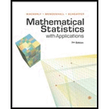
Mathematical Statistics with Applications
7th Edition
ISBN: 9780495110811
Author: Dennis Wackerly, William Mendenhall, Richard L. Scheaffer
Publisher: Cengage Learning
expand_more
expand_more
format_list_bulleted
Question
Chapter 6, Problem 94SE
To determine
Find the density
Expert Solution & Answer
Want to see the full answer?
Check out a sample textbook solution
Students have asked these similar questions
The work produced by a constant temperature, pressure - volume thermodynamic process can be computed as (picture 1)
where W is work, p is pressure, and V is volume. Use Simpson's rules to evaluate the work for the following data given in
TABLE picture.
Suppose that a given population can be divided into two parts: those who have a given disease and can infect others, and those who do not have it but are susceptible. Let x be the proportion of susceptible individuals and y the proportion of infectious individuals; then x + y = 1. Assume that the disease spreads by contact between sick and well members of the population and that the rate of spread dy/dt is proportional to the number of such contacts. Further, assume that members of both groups move about freely among each other, so the number of contacts is proportional to the product of x and y. Since x = 1 − y, we obtain the initial value problem
(22)
dydt=αy(1−y),y(0)=y0,where α is a positive proportionality factor, and y0 is the initial proportion of infectious individuals.
a.Find the equilibrium points for the differential equation (22) and determine whether each is asymptotically stable, semistable, or unstable.
b.Solve the initial value problem 22 and verify that the…
Find the population y(t) if the birth rate is
proportional to y(t) and the death rate is propors-
-tional to square of y(t).
Chapter 6 Solutions
Mathematical Statistics with Applications
Ch. 6.3 - Let Y be a random variable with probability...Ch. 6.3 - Prob. 2ECh. 6.3 - Prob. 3ECh. 6.3 - The amount of flour used per day by a bakery is a...Ch. 6.3 - Prob. 5ECh. 6.3 - The joint distribution of amount of pollutant...Ch. 6.3 - Suppose that Z has a standard normal distribution....Ch. 6.3 - Assume that Y has a beta distribution with...Ch. 6.3 - Prob. 9ECh. 6.3 - The total time from arrival to completion of...
Ch. 6.3 - Suppose that two electronic components in the...Ch. 6.3 - Prob. 12ECh. 6.3 - If Y1 and Y2 are independent exponential random...Ch. 6.3 - Prob. 14ECh. 6.3 - Prob. 15ECh. 6.3 - Prob. 16ECh. 6.3 - Prob. 17ECh. 6.3 - A member of the Pareto family of distributions...Ch. 6.3 - Prob. 19ECh. 6.3 - Let the random variable Y possess a uniform...Ch. 6.3 - Prob. 21ECh. 6.4 - Prob. 23ECh. 6.4 - In Exercise 6.4, we considered a random variable Y...Ch. 6.4 - Prob. 25ECh. 6.4 - Prob. 26ECh. 6.4 - Prob. 27ECh. 6.4 - Let Y have a uniform (0, 1) distribution. Show...Ch. 6.4 - Prob. 29ECh. 6.4 - A fluctuating electric current I may be considered...Ch. 6.4 - The joint distribution for the length of life of...Ch. 6.4 - Prob. 32ECh. 6.4 - The proportion of impurities in certain ore...Ch. 6.4 - A density function sometimes used by engineers to...Ch. 6.4 - Prob. 35ECh. 6.4 - Refer to Exercise 6.34. Let Y1 and Y2 be...Ch. 6.5 - Let Y1, Y2,, Yn be independent and identically...Ch. 6.5 - Let Y1 and Y2 be independent random variables with...Ch. 6.5 - Prob. 39ECh. 6.5 - Prob. 40ECh. 6.5 - Prob. 41ECh. 6.5 - A type of elevator has a maximum weight capacity...Ch. 6.5 - Prob. 43ECh. 6.5 - Prob. 44ECh. 6.5 - The manager of a construction job needs to figure...Ch. 6.5 - Suppose that Y has a gamma distribution with =...Ch. 6.5 - A random variable Y has a gamma distribution with ...Ch. 6.5 - Prob. 48ECh. 6.5 - Let Y1 be a binomial random variable with n1...Ch. 6.5 - Let Y be a binomial random variable with n trials...Ch. 6.5 - Prob. 51ECh. 6.5 - Prob. 52ECh. 6.5 - Let Y1,Y2,,Yn be independent binomial random...Ch. 6.5 - Prob. 54ECh. 6.5 - Customers arrive at a department store checkout...Ch. 6.5 - The length of time necessary to tune up a car is...Ch. 6.5 - Prob. 57ECh. 6.5 - Prob. 58ECh. 6.5 - Prob. 59ECh. 6.5 - Prob. 60ECh. 6.5 - Prob. 61ECh. 6.5 - Prob. 62ECh. 6.6 - In Example 6.14, Y1 and Y2 were independent...Ch. 6.6 - Refer to Exercise 6.63 and Example 6.14. Suppose...Ch. 6.6 - Prob. 65ECh. 6.6 - Prob. 66ECh. 6.6 - Prob. 67ECh. 6.6 - Prob. 68ECh. 6.6 - Prob. 71ECh. 6 - Let Y1 and Y2 be independent and uniformly...Ch. 6 - As in Exercise 6.72, let Y1 and Y2 be independent...Ch. 6 - Let Y1, Y2,, Yn be independent, uniformly...Ch. 6 - Prob. 75SECh. 6 - Prob. 76SECh. 6 - Prob. 77SECh. 6 - Prob. 78SECh. 6 - Refer to Exercise 6.77. If Y1,Y2,,Yn are...Ch. 6 - Prob. 80SECh. 6 - Let Y1, Y2,, Yn be independent, exponentially...Ch. 6 - Prob. 82SECh. 6 - Prob. 83SECh. 6 - Prob. 84SECh. 6 - Let Y1 and Y2 be independent and uniformly...Ch. 6 - Prob. 86SECh. 6 - Prob. 87SECh. 6 - Prob. 88SECh. 6 - Let Y1, Y2, . . . , Yn denote a random sample from...Ch. 6 - Prob. 90SECh. 6 - Prob. 91SECh. 6 - Prob. 92SECh. 6 - Prob. 93SECh. 6 - Prob. 94SECh. 6 - Prob. 96SECh. 6 - Prob. 97SECh. 6 - Prob. 98SECh. 6 - Prob. 99SECh. 6 - The time until failure of an electronic device has...Ch. 6 - Prob. 101SECh. 6 - Prob. 103SECh. 6 - Prob. 104SECh. 6 - Prob. 105SECh. 6 - Prob. 106SECh. 6 - Prob. 107SECh. 6 - Prob. 108SECh. 6 - Prob. 109SECh. 6 - Prob. 110SECh. 6 - Prob. 111SECh. 6 - Prob. 112SECh. 6 - Prob. 113SECh. 6 - Prob. 114SECh. 6 - Prob. 115SECh. 6 - Prob. 116SE
Knowledge Booster
Similar questions
- Table 6 shows the population, in thousands, of harbor seals in the Wadden Sea over the years 1997 to 2012. a. Let x represent time in years starting with x=0 for the year 1997. Let y represent the number of seals in thousands. Use logistic regression to fit a model to these data. b. Use the model to predict the seal population for the year 2020. c. To the nearest whole number, what is the limiting value of this model?arrow_forwardbThe average rate of change of the linear function f(x)=3x+5 between any two points is ________.arrow_forwardFind the constant of proportionality. y is directly proportional to x. If x=30, then y=15.arrow_forward
- When purifying drinking water you can use a so-called membrane filtration. In an experiment one wishes to examine the relationship between the pressure drop across a membrane and the flux (flow per area) through the membrane. We observe the following 10 related values of pressure (x) and flux (y): 1 2 3 4 5 7 8. 9 10 Pressure (x) 1.02 2.08 2.89 4.01 5.32 5.83 7.26 7.96 | 9.11 9.99 Flux (y) 1.15 0.85 1.56 1.72 4.32 5.07 5.00 5.31 6.17 7.04 (a) Fit the least square regression equation to predict the flux (flow per area) through the pressure drop across a membrane. (b) Find the estimated flux when the pressure drop across a membrane is 4.50. (c) Calculate the coefficient of correlation. Interpret your result. (d) Given Sxx = 83.25961 and Se = 0.64460653. Test, at the 0.01 level of significance, whether there is linear relationship between the pressure drop across a membrane and the flux (flow per area) through the membrane. (e) Construct a 98% confidence interval for the mean flux for the…arrow_forwardMist (airborne droplets or aerosols) is generated when metal-removing fluids are used in machining operations to cool and lubricate the tool and workpiece. Mist generation is a concern to OSHA, which has recently lowered substantially the workplace standard. An article gave the accompanying data on x = fluid-flow velocity for a 5% soluble oil (cm/sec) and y the extent of mist droplets having diameters smaller than 10 µm (mg/m³): 85 177 190 354 360 442 960 0.39 0.60 0.45 0.66 0.60 0.69 0.90 (a) The investigators performed a simple linear regression analysis to relate the two variables. Does a scatter plot of the data support this strategy? Yes, a scatter plot shows a reasonable linear relationship. No, a scatter plot does not show a reasonable linear relationship. (b) What proportion of observed variation in mist can be attributed to the simple linear regression relationship between velocity and mist? (Round your answer to three decimal places.) (c) The investigators were particularly…arrow_forward00 L[ft)= F(s) = [ e* f(1) dt -starrow_forward
- The efficiency for a steel specimen immersed in a phosphating tank is the weight of the phosphate coating divided by the metal loss (both in mg/ft). An article gave the accompanying data on tank temperature (x) and efficiency ratio (y). Temp. 171 173 174 175 175 176 177 178 Ratio 0.86 1.29 1.40 1.05 1.01 1.04 0.94 1.78 Temp. 181 181 181 181 181 182 182 183 Ratio 1.41 1.56 1.63 2.03 2.07 0.76 1.47 0.84 Temp. 183 183 183 185 185 186 187 189 Ratio 1.75 1.92 2.64 1.39 2.58 2.90 1.81 3.16 In USE SALT (a) Determine the equation of the estimated regression line. (Round all numerical values to four decimal places.) y = -15.3081 + 0.0939x (b) Calculate a point estimate for true average efficiency ratio when tank temperature is 183. (Round your answer to four decimal places.) 1.8756 (c) Calculate the values of the residuals from the least squares line for the four observations for which temperature is 183. (Round your answers to two decimal places.) (183, 0.84) |-1.03 (183, 1.75) |-0.12 (183,…arrow_forwardTrue or False If y varies directly with x, then y = k/x , where k is a constant.arrow_forwardThe flow rate of a pipe, Q in (m/s) is given by Q = dV where V is dt volume (in m) and t is time in (s). The volume in a pipe at time t is given in Table 1. Table 1 4 6 t, s 2 8 10 V(t), m3 7.56 3.87 5.09 6.34 4.59 Estimate the flow rate Q at time t = 4s by using: (a) 2-Point Forward Difference (b) 2-Point Backward Difference (c) 3-Point Central Differencearrow_forward
- Economists use Lorenz curves to illustrate the distribution of income in a country. A Lorenz curve, y = f(x), represents the actual income distribution in the country. In this model, x represents percents of families in the country from the poorest to the wealthiest and y represents percents of total income. The model y = x represents a country in which each family has the same income. The area between these two models, where 0 ≤ x ≤ 100, indicates a country’s “income inequality.” The table lists percents of income y for selected percents of families x in a country. (a) Use a graphing utility to find a quadratic model for the Lorenz curve. (b) Plot the data and graph the model. (c) Graph the model y = x. How does this model compare with the model in part (a)? (d) Use the integration capabilities of a graphing utility to approximate the “income inequality.”arrow_forwardthe edge of a cube was found to be 40cm w a possible error of .2cm. use differentials to estimate a. the max possible error regarding the cube’s volume b. the relative error in the volume of the cube c. the percentage error in the volume of the cubearrow_forwardU = Find values of u, a, b, and C so that a = [³³ b In (t³) t dt -fc = Cu du. C = =arrow_forward
arrow_back_ios
SEE MORE QUESTIONS
arrow_forward_ios
Recommended textbooks for you

 Functions and Change: A Modeling Approach to Coll...AlgebraISBN:9781337111348Author:Bruce Crauder, Benny Evans, Alan NoellPublisher:Cengage Learning
 Linear Algebra: A Modern IntroductionAlgebraISBN:9781285463247Author:David PoolePublisher:Cengage Learning
 Algebra and Trigonometry (MindTap Course List)AlgebraISBN:9781305071742Author:James Stewart, Lothar Redlin, Saleem WatsonPublisher:Cengage Learning
 Algebra & Trigonometry with Analytic GeometryAlgebraISBN:9781133382119Author:SwokowskiPublisher:Cengage


Functions and Change: A Modeling Approach to Coll...
Algebra
ISBN:9781337111348
Author:Bruce Crauder, Benny Evans, Alan Noell
Publisher:Cengage Learning

Linear Algebra: A Modern Introduction
Algebra
ISBN:9781285463247
Author:David Poole
Publisher:Cengage Learning

Algebra and Trigonometry (MindTap Course List)
Algebra
ISBN:9781305071742
Author:James Stewart, Lothar Redlin, Saleem Watson
Publisher:Cengage Learning


Algebra & Trigonometry with Analytic Geometry
Algebra
ISBN:9781133382119
Author:Swokowski
Publisher:Cengage