Control Systems Engineering
7th Edition
ISBN: 9781118170519
Author: Norman S. Nise
Publisher: WILEY
expand_more
expand_more
format_list_bulleted
Concept explainers
Videos
Textbook Question
Chapter 6, Problem 56P
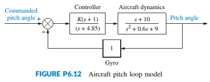
A model for an airplane’s pitch loop is shown in Figure P6.12. Find the range of gain, K, that will keep the system stable. Can the system ever be unstable for positive values of K?
Expert Solution & Answer
Want to see the full answer?
Check out a sample textbook solution
Students have asked these similar questions
4. A model for an airplane's pitch loop is shown below. Find the range of K that will keep the system stable.
Can the system every be unstable for positive values of K?
Commanded
pitch angle +
Controller
K(s + 1)
(s + 4.85)
1
Aircraft dynamics
s + 10
s² +0.6s +9
Gyro
Pitch angle
A satellite single-axis amplitude control system can be represented by the block diagram is
as shown in Figure 2.11. The variable k, a and b are controller parameters, andj is the
spacecraft moment of inertia. Suppose the moment of inertia is J=7.8E+08 (slug-ft), and the
controller parameters are k=10.8E+08, a=1.5 and b=8.
Spacecraft
Rotational
R(s)
Controller
motion
C(s)
k(s + a)
(s + b)
js?
Figure 2.11 A negative feedback control system
a) Develop an m-file script to compute the closed loop transfer function.
b) Compute and plot the step response to a 10° step input.
c) The exact moment of inertia is generally unknown and any change slowly with time.
Compare the step response performance of the spacecraft when J is reduced by 25%
and 60%.
2. A model for an airplane's pitch loop is shown below. Find the range of K that will keep the system
stable. Can the system ever be unstable for positive values of K?
Controller
Aircraft dynamics
Commanded
pitch angle +
K(s + 1)
Pitch angle
s + 10
s2 + 0.6s + 9
(s + 4.85)
1
Gyro
Chapter 6 Solutions
Control Systems Engineering
Ch. 6 - Prob. 1RQCh. 6 - Prob. 2RQCh. 6 - What would happen to a physical system chat...Ch. 6 - Why are marginally stable systems considered...Ch. 6 - Prob. 5RQCh. 6 - Prob. 6RQCh. 6 - Prob. 7RQCh. 6 - Prob. 8RQCh. 6 - Prob. 9RQCh. 6 - Why do we sometimes multiply a row of a Routh...
Ch. 6 - Prob. 11RQCh. 6 - Prob. 12RQCh. 6 - 13. Does the presence of an entire row of zeros...Ch. 6 - Prob. 14RQCh. 6 - Prob. 15RQCh. 6 - Prob. 16RQCh. 6 - Tell how many roots of the following polynomial...Ch. 6 - Tell how many roots of the following polynomial...Ch. 6 - Using the Routh table, tell how many poles of the...Ch. 6 - Prob. 4PCh. 6 - Determine how many closed-loop poles lie in the...Ch. 6 - Determine how many closed-loop poles lie in the...Ch. 6 - MATLAB ML 7. Use MATLAB to find the pole location...Ch. 6 - Symbolic Math SM 8. Use MATLAB and the Symbolic...Ch. 6 - Determine whether the unity feedback system of...Ch. 6 - Use MATLAB to find the pole locations for the...Ch. 6 - Consider the unity feedback system of Figure P6.3...Ch. 6 - In the system of Figure P6.3, let Gs=Ks+1ss2s+3...Ch. 6 - Given the unity feedback system of Figure P6.3...Ch. 6 - Using the Routh-Hurwitz criterion and the unity...Ch. 6 - Given the unity feedback system of Figure P6.3...Ch. 6 - Repeat Problem 15 using MATLAB.Ch. 6 - Prob. 17PCh. 6 - For the system of Figure P6.4, tell how many...Ch. 6 - Using the Routh-Hurwitz criterion, tell how many...Ch. 6 - Determine if the unity feedback system of Figure...Ch. 6 - For the unity feedback system of Figure P6.3 with...Ch. 6 - In the system of Figure P6.3, let Gs=Ksassb Find...Ch. 6 - For the unity feedback system of Figure P63 with...Ch. 6 - Find the range of K for stability for the unity...Ch. 6 - For the unity feedback system of Figure P6.3 with...Ch. 6 - find the range of K for stability. [Section: 6.41]...Ch. 6 - Find the range of gain, K, to ensure stability in...Ch. 6 - Using the Routh-Hurwitz criterion, find the value...Ch. 6 - Use the Routh-Hurwitz criterion to find the range...Ch. 6 - Prob. 32PCh. 6 - Given the unity feedback system of Figure P63 with...Ch. 6 - Repeat Problem 33 for [Section: 6.4]...Ch. 6 - For the system shown in Figure P6.8, find the...Ch. 6 - Given the unity feedback system of Figure P6.3...Ch. 6 - For the unity feedback system of Figure P6.3 with...Ch. 6 - For the unity feedback system of Figure P6.3 with...Ch. 6 - Given the unity feedback system of Figure P6.3...Ch. 6 - Using the Routh-Hurwitz criterion and the unity...Ch. 6 - Find the range of K to keep the system shown in...Ch. 6 - Prob. 43PCh. 6 - The closed-loop transfer function of a system is...Ch. 6 - Prob. 45PCh. 6 - Prob. 46PCh. 6 - An interval polynomial is of the form...Ch. 6 - A linearized model of a torque-controlled crane...Ch. 6 - The read/write head assembly arm of a computer...Ch. 6 - A system is represented in state space as...Ch. 6 - State Space SS 52. The following system in state...Ch. 6 - Prob. 54PCh. 6 - A model for an airplane’s pitch loop is shown in...Ch. 6 - Prob. 57PCh. 6 - Prob. 58PCh. 6 - Prob. 59PCh. 6 - Prob. 60PCh. 6 - Prob. 61PCh. 6 - Look-ahead information can be used to...Ch. 6 - Prob. 63PCh. 6 - It has been shown (Pounds, 2011) that an unloaded...Ch. 6 - Prob. 65PCh. 6 - The system shown in Figure P6.16 has G1s=1/ss+2s+4...Ch. 6 - Prob. 67PCh. 6 - Prob. 68PCh. 6 - Hybrid vehicle. Figure P6.l8 shows the HEV system...Ch. 6 - Prob. 70P
Knowledge Booster


Learn more about
Need a deep-dive on the concept behind this application? Look no further. Learn more about this topic, mechanical-engineering and related others by exploring similar questions and additional content below.Similar questions
- Consider in Figure 1 = 0. Iff, the translational mechanical system shown P4.17. A 1-pound force, f(t), is applied at 1, find K and M such that the response is characterized by a 4-second settling time and a 1-second peak time. Also, what is the resulting percent overshoot? [Section: 4.6] 1+ 270 Karrow_forwardA certain mass is driven by base excitation through a spring (Figure P4.13). Its parameter values are m = 100 kg, c = 1000 N * s/m, and k = 10,000 N/m. Determine its peak frequency w_p, it’s peak M_p, and its bandwidth.arrow_forwardThe state X(t) of a dynamical system is solution of equation 10x (t) + 30ax(t) = 40, with a = 13. Calculate the rise time of the response.arrow_forward
- Figure Q3 shows one cart with a mass that is separated from two walls by two springs and a dashpot, where kı, k2 and ka are the first, second spring and dashpot coefficients, respectively. The mass, m could represent an automobile system. An external force is also shown as F(t). Only horizontal motion and forces are considered. F(t) is input and x2(t) is output. (a) Derive all equations related to the system (b) Construct the block diagram from equation in (a) (c) Obtain the transfer function of the systemarrow_forwardWhat is the step response of the dynamic system pictured below?arrow_forwardA machine weighing 2000 N rests on a support as illustrated in Figure P2.37. The support deflects about 5 cm as a result of the weight of the machine. The floor under the support is somewhat flexible and moves, because of the motion of a nearby machine, harmonically near resonance (r=1) with an amplitude of 0.2 cm. Model the floor as base motion, and assume a damping ratio of = 0.01, and calculate the transmitted force and the amplitude of the transmitted displacement. 2.37 Machine of mass m Rubber mount modeled as a A = static deflection stiffness k and a damper c Flexible floor y(t) Figure P2.37arrow_forward
- Example # 1 For the mechanical system shown, a force of 2 lb( step input) is applied to the system, the mass oscillates, as shown in fig. determi from this response curve. The displacement x is measured from the equilibrium position m, b, k of the system 0.0095 ft 0.1 ft 4 5 (b)arrow_forwardFor the system shown in the figure: b V f(t) a) Find the mathematical model of the system b) Consider null initial conditions, f(t)=1 N₁ m=1 Kg and find values of k and b for the position x(t) to show the following responses: Sustained oscillations • Attenuated oscillations No oscillations c) Obtain an analog simulation diagram and use Simulink to solve the system c) Plot the position x(t) for the 3 cases in point (b)arrow_forwardA mass of 2 kilograms is on a spring with spring constant k newtons per meter with no damping. Suppose the system is at rest and at time t = 0 the mass is kicked and starts traveling at 2 meters per second. How large does k have to be to so that the mass does not go further than 3 meters from the rest position? use 2nd order differential equations to solve (mechanical vibrations)arrow_forward
- For the system shown in Figure, find: a) The system equation of motion in terms of θ b) The system natural frequency, ωn c) The system damping factor, ξ d)The system natural damped frequencyarrow_forwardShips at sea undergo motion about their roll axis, as shown in Fig. The stabilizers can be positioned by a closed-loop roll control system that consists of components, such as fin actuators and sensors, as well as the ship's roll dynamics. Assume the roll dynamics, which relates the roll-angle output, θ(s), to a disturbance-torque input, TD(s) Find the natural frequency, damping ratio, peak time and percent overshoot. Question 5 options: ωn=2.8 rad/s, ξ=0.5Peak time 5.12sOvershoot 69.26% ωn=0.5 rad/s, ξ=2.25Peak time 4.16sOvershoot 49.1% ωn=2.25 rad/s, ξ=0.5Peak time 3.45sOvershoot 30.85%arrow_forwardFor the system shown in the figure below: 1. Derive the system differential equations of motion. 2. Use Laplace transform to solve for the displacement x:(t) and x2(t), when K,=k2 =k3=1, m,= m;=1, and x1(0) =0, x1(0) = -1, x2(0) =0, and x{0) =1 3. Sketch x:(t) and X2(t) m, X1 X2arrow_forward
arrow_back_ios
SEE MORE QUESTIONS
arrow_forward_ios
Recommended textbooks for you
 Elements Of ElectromagneticsMechanical EngineeringISBN:9780190698614Author:Sadiku, Matthew N. O.Publisher:Oxford University Press
 Mechanics of Materials (10th Edition)Mechanical EngineeringISBN:9780134319650Author:Russell C. HibbelerPublisher:PEARSON
 Thermodynamics: An Engineering ApproachMechanical EngineeringISBN:9781259822674Author:Yunus A. Cengel Dr., Michael A. BolesPublisher:McGraw-Hill Education
 Control Systems EngineeringMechanical EngineeringISBN:9781118170519Author:Norman S. NisePublisher:WILEY
 Mechanics of Materials (MindTap Course List)Mechanical EngineeringISBN:9781337093347Author:Barry J. Goodno, James M. GerePublisher:Cengage Learning
 Engineering Mechanics: StaticsMechanical EngineeringISBN:9781118807330Author:James L. Meriam, L. G. Kraige, J. N. BoltonPublisher:WILEY
Elements Of Electromagnetics
Mechanical Engineering
ISBN:9780190698614
Author:Sadiku, Matthew N. O.
Publisher:Oxford University Press
Mechanics of Materials (10th Edition)
Mechanical Engineering
ISBN:9780134319650
Author:Russell C. Hibbeler
Publisher:PEARSON
Thermodynamics: An Engineering Approach
Mechanical Engineering
ISBN:9781259822674
Author:Yunus A. Cengel Dr., Michael A. Boles
Publisher:McGraw-Hill Education
Control Systems Engineering
Mechanical Engineering
ISBN:9781118170519
Author:Norman S. Nise
Publisher:WILEY
Mechanics of Materials (MindTap Course List)
Mechanical Engineering
ISBN:9781337093347
Author:Barry J. Goodno, James M. Gere
Publisher:Cengage Learning
Engineering Mechanics: Statics
Mechanical Engineering
ISBN:9781118807330
Author:James L. Meriam, L. G. Kraige, J. N. Bolton
Publisher:WILEY
Introduction to Undamped Free Vibration of SDOF (1/2) - Structural Dynamics; Author: structurefree;https://www.youtube.com/watch?v=BkgzEdDlU78;License: Standard Youtube License