Concept explainers
Videos
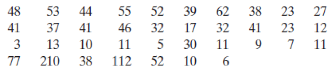
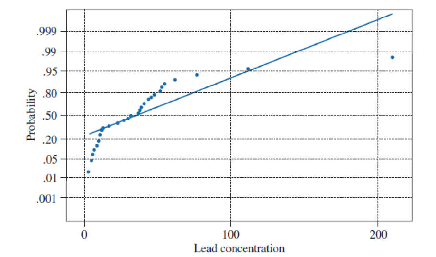
The vulnerability of inshore environments to contamination due to urban and industrial expansion in Mombasa is discussed in the paper “Metals, Petroleum Hydrocarbons and Organochlorines in Inshore Sediments and Waters on Mombasa, Kenya” [Marine Pollution Bulletin (1997) 34:570–577]. A geochemical and oceanographic survey of the inshore waters of Mombasa, Kenya, was undertaken during the period from September 1995 to January 1996. In the survey, suspended particulate matter and sediment were collected from 48 stations within Mombasa’s estuarine creeks. The concentrations of major oxides and 13 trace elements were determined for a varying number of cores at each of the stations. In particular, the lead concentrations in suspended particulate matter (mg kg−1 dry weight) were determined at 37 stations. The researchers were interested in determining whether the average lead concentration was greater than 30 mg kg−1 dry weight. The data are given in the following table along with summary statistics and a normal
Lead concentrations (mg kg−1 dry weight) from 37 stations in Kenya
- a. Is there sufficient evidence (α = .05) in the data that the mean lead concentration exceeds 30 mg kg−1 dry weight?
- b. What is the probability of a Type II error if the actual mean concentration is 50?
- c. Do the data appear to have a
normal distribution ? - d. Based on your answer in (c), is the
sample size large enough for the test procedures to be valid? Explain.
Want to see the full answer?
Check out a sample textbook solution
Chapter 5 Solutions
An Introduction to Statistical Methods and Data Analysis


- The vulnerability of inshore environments to contamination due to urban and industrial expansion in Mombasa is discussed in the paper “Metals, Petroleum Hydrocarbons and Organo- chlorines in Inshore Sediments and Waters on Mombasa, Kenya” [Marine Pollution Bulletin (1997) 34:570–577]. A geochemical and oceanographic survey of the inshore waters of Mombasa, Kenya, was undertaken during the period from September 1995 to January 1996. In the survey, suspended particulate matter and sediment were collected from 48 stations within Mombasa’s estuarine creeks. The concentrations of major oxides and 13 trace elements were determined for a varying number of cores at each of the stations. In particular, the lead concentrations in sus-pended particulate matter (mg kg21 dry weight) were determined at 37 stations. The researchers were interested in determining whether the average lead concentration was greater than 30 mg kg21 dry weight. The data are given in the following table along with summary…arrow_forwardThe article "Oxidation State and Activities of Chromium Oxides in Cao-SiO,-CrO, Slag System" (Y. Xiao, L. Holappa, and M. Reuter, Metallurgical and Materials Transactions B, 2002:595-603) presents the amount x (in mole percent) and activity coefficient y of CrO,5 for several specimens. The data, extracted from a larger table, are presented in the following table. х У 2.6 10.20 5.03 19.9 8.84 0.8 6.62 5.3 2.89 20.3 2.31 39.4 7.13 5.8 3.40 29.4 5.57 2.2 7.23 5.5 2.12 33.1 1.67 44.2 5.33 13.1 16.70 0.6 9.75 2.2 2.74 16.9 2.58 35.5 1.50 48.0 Compute the least-squares line for predicting y from x. b. Plot the residuals versus the fitted values. Compute the least-squares line for predicting y from 1/x. d. Plot the residuals versus the fitted values. C. Using the better fitting line, find a 95% confidence interval for the mean value of y when x= 5.0.arrow_forwardThe depth of wetting of a soil is the depth to which water content will increase owing to extemal factors. The article "Discussion of Method for Evaluation of Depth of Wetting in Residential Areas" (J. Nelson, K. Chao, and D. Overton, Journal of Geotechnical and Geoenvironmental Engineering, 2011:293-296) discusses the relationship between depth of wetting beneath a structure and the age of the structure. The article presents measurements of depth of wetting, in meters, and the ages, in years, of 21 houses, as shown in the following table. Age Depth 7.6 4 4.6 6.1 9.1 3 4.3 7.3 5.2 10.4 15.5 5.8 10.7 4 5.5 6.1 10.7 10.4 4.6 7.0 6.1 14 16.8 10 9.1 8.8 Compute the least-squares line for predicting depth of wetting (y) from age (x). b. Identify a point with an unusually large x-value. Compute the least-squares line that results from deletion of this point. Identify another point which can be classified as an outlier. Compute the least-squares line that results from deletion of the outlier,…arrow_forward
- Please use the accompanying Excel data set or accompanying Text file data set when completing the following exercise. An article in Urban Ecosystems, "Urbanization and Warming of Phoenix (Arizona, USA): Impacts, Feedbacks and Mitigation" (2002, Vol. 6, pp. 183–203), mentions that Phoenix is ideal to study the effects of an urban heat island because it has grown from a population of 300,000 to approximately 3 million over the last 50 years and this is a period with a continuous, detailed climate record. The 50-year averages of the mean annual temperatures at eight sites in Phoenix are shown below. Check the assumption of normality in the population with a probability plot. Construct a 95% confidence interval for the standard deviation over the sites of the mean annual temperatures. Site Sky Harbor Airport 23.3 Average Mean Temperature (°C) Phoenix Greenway 21.7 Phoenix Encanto Waddell 21.6 21.7arrow_forward7. The article "Hydrogeochemical Characteristics of Groundwater in a Mid-Western Coastal Aquifer System" (S. Jeen, J. Kim, et al., Geosciences Journal, 2001:339-348) presents measurements of various properties of shallow groundwater in a certain aquifer system in Korea. Following are measurements of electrical conductivity (in microsiemens per centimeter) for 23 water samples. 2099 528 2030 1350 1018 384 1499 1265 375 424 789 810 522 513 488 200 215 486 257 557 260 461 500 a. Find the mean. b. Find the standard deviation. c. Find the median. d. Findthe 10%trimmedmean. e. Find the first quartile. f. Find the third quartile. g. Find the interquartile range. h. Construct a boxplot. i. Which of the points, if any, are outliers? j. If a histogram were constructed, would it be skewed to the left, skewed to the right, or approximately symmetric? 8. Forty-five specimens of a certain type of powder were analyzed for sulfur trioxide content. Following are the results, in percent. The list has…arrow_forwardThe following table shows the typical depth (rounded to the nearest foot) for nonfailed wells in geological formations in Baltimore County (The Journal of Data Science, 2009, Vol. 7, pp. 111-127). Geological Formation Group Number of Nonfailed Wells Nonfailed Well Depth Gneiss 1,515 255 Granite 26 218 Loch Raven Schist 3,290 317 Mafic 349 231 Marble 280 267 Prettyboy Schist 1,343 255 Other schists 887 267 Serpentine 36 217 Total 7,726 2,027 Let the random variable X denote the depth (rounded to the nearest foot) for nonfailed wells. Detemine the cumulative distribution function for X. Round your answers to four decimal places (e.g. 98.7654). x < 217 217arrow_forwardThe Great White Shark. In an article titled “Great White, Deep Trouble” (National Geographic, Vol. 197(4), pp. 2–29), Peter Benchley—the author of JAWS—discussed various aspects of the Great White Shark (Carcharodon carcharias). Data on the number of pups borne in a lifetime by each of 80 Great White Shark females are provided on the WeissStats site. a. obtain and interpret the quartiles. b. determine and interpret the interquartile range. c. find and interpret the five-number summary. d. identify potential outliers, if any. e. obtain and interpret a boxplot.arrow_forwardThe article "Hydrogeochemical Characteristics of Groundwater in a Mid-Western Coastal Aquifer System" (S. Jeen, J. Kim, et al., Geosciences Journal, 2001:339-348) presents measurements of various properties of shallow groundwater in a certain aquifer system in Korea. Following are measurements of electrical conductivity (in microsiemens per centimeter) for 23 water samples. 2099 528 2030 1350 1018 384 1499 1265 375 424 789 810 522 513 488 200 215 486 257 557 260 461 500 a) Find the mean, median, mode, and standard deviation. b) Construct a histogram using relative frequency on the y-axis and comment on the shape of the distribution.arrow_forwardPlease use the accompanying Excel data set or accompanying Text file data set when completing the following exercise. An article in Urban Ecosystems, "Urbanization and Warming of Phoenix (Arizona, USA): Impacts, Feedbacks and Mitigation" (2002, Vol. 6, pp. 183-203), mentions that Phoenix is ideal to study the effects of an urban heat island because it has grown from a population of 300,000 to approximately 3 million over the last 50 years and this is a period with a continuous, detailed climate record. The 50-year averages of the mean annual temperatures at eight sites in Phoenix are shown below. Check the assumption of normality in the population with a probability plot. Construct a 95% confidence interval for the standard deviation over the sites of the mean annual temperatures. Site Sky Harbor Airport 23.3 Phoenix Greenway 21.7 Phoenix Encanto 21.6 Waddell Litchfield Laveen Average Mean Temperature (°C) Maricopa Harlquahala i 21.7 21.3 20.7 20.9 20.1 Round the answers to three…arrow_forwardArchaeologists can determine the diets of ancient civilizations by measuring the ratio of carbon-13 to carbon-12 in bones found at burial sites. Large amounts of carbon-13 suggest a diet rich in grasses such as maize, while small amounts suggest a diet based on herbaceous plants. The article "Climate and Diet in Fremont Prehistory: Economic Variability and Abandonment of Maize Agriculture in the Great Salt Lake Basin" (J. Coltrain and S. Leavitt, American Antiquity, 2002:453-485) reports ratios, as a difference from a standard in units of parts per thousand, for bones from individuals in several age groups. The data are presented in the following table. Ratio Age Group (years) 0-11 17.2 18.4 17.9 16.6 19.0 18.3 13.6 13.5 18.5 19.1 19.1 13.4 12-24 14.8 17.6 18.3 17.2 10.0 11.3 10.2 17.0 18.9 19.2 25-45 18.4 13.0 14.8 18.4 12.8 17.6 18.8 179 18.5 17.5 18.3 15.2 10.8 19.8 1 19.2 15.4 13.2 46+ 15.5 18.2 12.7 15.1 18.2 18.0 14.4 10.2 16.7 Construct an ANOVA table. You may give a range for…arrow_forwardThe article "Mathematical Modeling of the Argon-Oxygen Decarburization Refining Process of Stainless Steel: Part II. Application of the Model to Industrial Practice" (J. Wei and D. Zhu, Metallurgical and Materials Transactions B, 2001:212-217) presents the carbon content (in mass %) and bath temperature (in K) for 32 heats of austenitic stainless steel. These data are shown in the following table. Carbon % Temp. 1975 19 23 1947 22 1954 16 1992 17 1965 18 1971 12 2046 24 1945 17 1984 20 1991arrow_forward4. A study to assess the capability of subsurface flow wetland systems to remove biochemical oxygen demand (BOD) and various other chemical constituents resulted in the accompanying data on z = BOD mass loading (kg/ha/d) and y = BOD mass removal (kg/ha/d) ("Subsurface Flow Wetlands-A Performance Evaluation." Water Envir. Res., 1995: 244-247). x Y 11 8 13 16 27 10 11 16 142 35 38 44 103 30 90 75 31 30 26 21 n = 10; Σ | n = 450; Σα" = 37653; Σy = 318; Σ y = 17244; Σ =y = 25344 Answer the following questions: (a) Plot an appropriate graph for the data. (b) Obtain the best lincar prediction equation. (c) For every additional unit change in BOD mass loading, by how much does the BOD mass removal change, on average? (d) Give the value of the statistic that measures the linear association between the BOD mass loading and BOD mass removal. Comment. (e) What percent of variation in the BOD mass removal is explained by the variation by the BOD mass loading? (f) Predict the BOD mass removal,…arrow_forwardarrow_back_iosSEE MORE QUESTIONSarrow_forward_ios
 MATLAB: An Introduction with ApplicationsStatisticsISBN:9781119256830Author:Amos GilatPublisher:John Wiley & Sons Inc
 Probability and Statistics for Engineering and th...StatisticsISBN:9781305251809Author:Jay L. DevorePublisher:Cengage Learning
 Statistics for The Behavioral Sciences (MindTap C...StatisticsISBN:9781305504912Author:Frederick J Gravetter, Larry B. WallnauPublisher:Cengage Learning
 Elementary Statistics: Picturing the World (7th E...StatisticsISBN:9780134683416Author:Ron Larson, Betsy FarberPublisher:PEARSON
 The Basic Practice of StatisticsStatisticsISBN:9781319042578Author:David S. Moore, William I. Notz, Michael A. FlignerPublisher:W. H. Freeman
 Introduction to the Practice of StatisticsStatisticsISBN:9781319013387Author:David S. Moore, George P. McCabe, Bruce A. CraigPublisher:W. H. Freeman