
Videos
Determine the roots of
(a)
To calculate: The real roots of the equation
Answer to Problem 4P
Solution: Graphically, the real roots of the equation are approximated as
Explanation of Solution
Given Information: The equation
Formula used: The roots of an equation can be represented graphically by the x-coordinate of the point where the graph intercepts the x-axis.
Calculation:
Use the following MATLAB code to plot the function
Execute the above code to obtain the plot as,
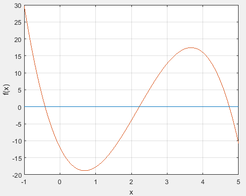
From the plot, the zeros of the equation are approximated as
(b)
To calculate: The root of the equation
Answer to Problem 4P
Solution: The root of the equation is approximated as
Explanation of Solution
Given Information: The function equation is
Initial guesses are,
Formula used: A root of an equation can be obtained using the bisection method as follows:
1. Choose two values of x, say a and b such that
2. Estimate the root by
3. If,
Calculation:
For the function
Thus,
Calculate the first root to be,
Further,
Thus,
Calculate the second root to be:
The approximate error is computed as:
Therefore, the approximate relative percentage error is 100%.
Furthermore,
Thus,
Calculate the third root to be:
The approximate error is computed as:
The approximate error is 33.3%.
Further,
Thus,
Calculate the fourth root to be:
The approximate error is computed as:
The approximate error is 14.28%.
Thus,
Therefore,
Calculate the fifth root to be:
The approximate error is computed as:
The approximate error is 7.69%.
Thus,
Therefore,
Calculate the sixth root to be:
The approximate error is computed as:
The approximate error is 3.7%.
Thus,
Therefore,
Calculate the seventh root to be:
The approximate error is computed as:
The approximate error is 1.89%.
Further,
Thus,
Calculate the eighth root to be:
The approximate error is computed as:
The approximate error is 0.93%.
As,
(c)
To calculate: The root of the equation
Answer to Problem 4P
Solution: The root of the equation can be approximated as
Explanation of Solution
Given Information: The equation
Initial guesses are,
Formula used: A root of an equation can be obtained using the false-position method as follows:
1. Choose two values of x, say a and b such that
2. Estimate the root by
3. If,
Calculation:
For the function
Thus,
Calculate the first root to be,
Now,
Thus,
Calculate the second root to be:
The approximate error is computed as:
The approximate relative percentage error is 24.25%.
Further,
Thus,
Calculate the third root to be:
The approximate error is computed as:
The approximate error is 6.36%.
Now,
Thus,
Calculate the fourth root to be:
The approximate error is computed as:
The approximate error is 1.68%.
Now,
Thus,
Calculate the fifth root would be:
The approximate error is computed as:
The approximate error is 0.45%.
As,
Want to see more full solutions like this?
Chapter 5 Solutions
EBK NUMERICAL METHODS FOR ENGINEERS
Additional Engineering Textbook Solutions
Fundamentals of Differential Equations (9th Edition)
Basic Technical Mathematics
Advanced Engineering Mathematics
An Introduction to Mathematical Statistics and Its Applications (6th Edition)
Geometry For Enjoyment And Challenge


- 2-the pivot value is the point of the intersection of the row of the leaving variable and the column of the solution. * true falsearrow_forwardThe natural exponential function can be expressed by . Determine e2by calculating the sum of the series for:(a) n = 5, (b) n = 15, (c) n = 25For each part create a vector n in which the first element is 0, the incrementis 1, and the last term is 5, 15, or 25. Then use element-by-element calculations to create a vector in which the elements are . Finally, use the MATLAB built-in function sum to add the terms of the series. Compare thevalues obtained in parts (a), (b), and (c) with the value of e2calculated byMATLAB.arrow_forwardf(x)=-0.9x? +1.7x+2.5 Calculate the root of the function given below: a) by Newton-Raphson method b) by simple fixed-point iteration method. (f(x)=0) Use x, = 5 as the starting value for both methods. Use the approximate relative error criterion of 0.1% to stop iterations.arrow_forward
- Problem #3 Determine the roots of f (x) =-12 – 21x + 18x² – 2.75x³ using the false-position method, with initial guesses of xi=-1 and xu = 0 and a stopping criterion of 1%. f(xu)(xl – xu) f(x1) – f(xu) X, = xu –arrow_forwardfor 0 < x < 1 у (х) %3 Зех - 5 Use the Bisection Method to look for a root of the equation. Begin with values of x = 0.5 and = 0.6. Complete three iterations of the method by filling out the table below. Show your %3D calculations. Xc f(x,) f (x.) Iterations Xr 1 0.5 0.8arrow_forwardmathforadmi..2dff1dd723 PTU Kadoorie sygini 1930 Technical Department of Applied Mathematics Second Semester 2020/2021 Math for Administration Assignment 2 Question 1 For the function: y = 0.01x- 0.001x² Find the zeros, the vertex and the optimum value (max. or min.) Question 2 Suppose a company has fixed costs of $300 and variable 3 costs of x + 1460 dollars per unit, 4 where x is the total number of units produced. Suppose further that the selling price of its product is 1500 X- ♡ lar Fine break-even points. init. II جامعة Palestine ||arrow_forward
- For the equation: a. Secant Method. Use Secant Method to determine the root of the given function up to three iterations use x_1= 0 and xo = 2. Complete the table using the HAND Calculation. Maintain 6 decimal places XH ex = 3 f(x+1) X₁ f(x₁) Eaarrow_forwardSelect the graph showing Tmax versus D1 after answering the question.arrow_forward3. Using the trial function u¹(x) = a sin(x) and weighting function w¹(x) = b sin(x) find an approximate solution to the following boundary value problems by determining the value of coefficient a. For each one, also find the exact solution using Matlab and plot the exact and approximate solutions. (One point each for: (i) finding a, (ii) finding the exact solution, and (iii) plotting the solution) a. (U₁xx -2 = 0 u(0) = 0 u(1) = 0 b. Modify the trial function and find an approximation for the following boundary value problem. (Hint: you will need to add an extra term to the function to make it satisfy the boundary conditions.) (U₁xx-2 = 0 u(0) = 1 u(1) = 0arrow_forward
- For the DE: dy/dx=2x-y y(0)=2 with h=0.2, solve for y using each method below in the range of 0 <= x <= 3: Q1) Using Matlab to employ the Euler Method (Sect 2.4) Q2) Using Matlab to employ the Improved Euler Method (Sect 2.5 close all clear all % Let's program exact soln for i=1:5 x_exact(i)=0.5*i-0.5; y_exact(i)=-x_exact(i)-1+exp(x_exact(i)); end plot(x_exact,y_exact,'b') % now for Euler's h=0.5 x_EM(1)=0; y_EM(1)=0; for i=2:5 x_EM(i)=x_EM(i-1)+h; y_EM(i)=y_EM(i-1)+(h*(x_EM(i-1)+y_EM(i-1))); end hold on plot (x_EM,y_EM,'r') % Improved Euler's Method h=0.5 x_IE(1)=0; y_IE(1)=0; for i=2:1:5 kA=x_IE(i-1)+y_IE(i-1); u=y_IE(i-1)+h*kA; x_IE(i)=x_IE(i-1)+h; kB=x_IE(i)+u; k=(kA+kB)/2; y_IE(i)=y_IE(i-1)+h*k; end hold on plot(x_IE,y_IE,'k')arrow_forward2. Answer the question completely and write down the given, required and formula that had been used. Provide graph and accurate/comple solution. The value are: V- 1 X- 5 W- 7 Y- 6 Z- 8arrow_forward3. Using the trial function uh(x) = a sin(x) and weighting function wh(x) = b sin(x) find an approximate solution to the following boundary value problems by determining the value of coefficient a. For each one, also find the exact solution using Matlab and plot the exact and approximate solutions. (One point each for: (i) finding a, (ii) finding the exact solution, and (iii) plotting the solution) a. (U₁xx - 2 = 0 u(0) = 0 u(1) = 0 b. Modify the trial function and find an approximation for the following boundary value problem. (Hint: you will need to add an extra term to the function to make it satisfy the boundary conditions.) (U₁xx - 2 = 0 u(0) = 1 u(1) = 0arrow_forward
 Elements Of ElectromagneticsMechanical EngineeringISBN:9780190698614Author:Sadiku, Matthew N. O.Publisher:Oxford University Press
 Mechanics of Materials (10th Edition)Mechanical EngineeringISBN:9780134319650Author:Russell C. HibbelerPublisher:PEARSON
 Thermodynamics: An Engineering ApproachMechanical EngineeringISBN:9781259822674Author:Yunus A. Cengel Dr., Michael A. BolesPublisher:McGraw-Hill Education
 Control Systems EngineeringMechanical EngineeringISBN:9781118170519Author:Norman S. NisePublisher:WILEY
 Mechanics of Materials (MindTap Course List)Mechanical EngineeringISBN:9781337093347Author:Barry J. Goodno, James M. GerePublisher:Cengage Learning
 Engineering Mechanics: StaticsMechanical EngineeringISBN:9781118807330Author:James L. Meriam, L. G. Kraige, J. N. BoltonPublisher:WILEY