
Videos
Determine the real roots of
(a) Graphically.
(b) Using the
(c) Using three iterations of the bisection method to determine the highest root. Employ initial guesses of
Compute the estimated error
(a)
The real roots of the equation
Answer to Problem 1P
Solution:
The real roots of the equation are
Explanation of Solution
Given Information:
The equation
Calculation:
The graph of the function can be plotted using MATLAB.
Code:
Output:
This gives the following plot:
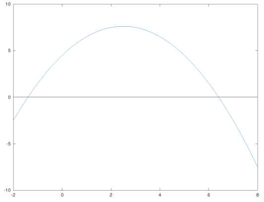
The roots of an equation can be represented graphically by the x-coordinate of the point where the graph cuts the x-axis. From the plot, the two zeros of the equation can be approximated as
(b)
To calculate: The real roots of the equation
Answer to Problem 1P
Solution:
The roots of the equation are
Explanation of Solution
Given Information:
The equation
Formula Used:
The roots of an equation
Calculation:
Consider the provided equation,
Now substitute
Thus, the roots of the equation are
(c)
To calculate: The highest root of the equation
Answer to Problem 1P
Solution:
The highest root of the equation can be approximated as 6.875. The true and approximate errors are as follows:
Explanation of Solution
Given Information:
The equation
Formula Used:
A root of an equation can be obtained using the bisection method as follows:
1. Choose 2 values x, say a and b such that
2. Now, estimate the root by
3. If,
Calculation:
For the provided function:
Hence,
Now take the first root to be,
As, the true root computed from part (b) was 6.40512484. Now, the true relative percentage error would be:
The true error is 17.1%. There would be no approximate error for the first iteration.
Now,
Thus,
Now, the second root would be:
As, the true root computed from part (b) was 6.40512484. Now, the true relative percentage error would be:
The true error is 2.42%.
The approximate error can be computed as:
The approximate error is 2%.
Now,
Thus,
Now, the third root would be:
As, the true root computed from part (b) was 6.40512484. Now, the true relative percentage error would be:
The true error is 7.34%.
The approximate error can be computed as:
The approximate error is 9.09%.
Thus, the highest root can be approximated as 6.875.
Want to see more full solutions like this?
Chapter 5 Solutions
EBK NUMERICAL METHODS FOR ENGINEERS


- The natural exponential function can be expressed by . Determine e2by calculating the sum of the series for:(a) n = 5, (b) n = 15, (c) n = 25For each part create a vector n in which the first element is 0, the incrementis 1, and the last term is 5, 15, or 25. Then use element-by-element calculations to create a vector in which the elements are . Finally, use the MATLAB built-in function sum to add the terms of the series. Compare thevalues obtained in parts (a), (b), and (c) with the value of e2calculated byMATLAB.arrow_forwardA root of the function f(x) = x3 – 10x² +5 lies close to x = 0.7. Doing three iterations, compute this root using the Newton- Raphson method with an initial guess of x=1). Newton-Raphson iterative equation is given as: f(x;) Xi+1 = Xị - f'(xi)arrow_forward8. Use the Lagrange multiplier method to find the point on the line 3x + 8y = 146 that is closest to the origin.arrow_forward
- Use a step size of 0.1 and round your answers to five decimal places if needed. Use Euler's method to approximate the solution x10 for the IVP y' 8y, y(0) 1. The Euler approximation for x10 isarrow_forwardby using simple iteration method find one root of the following equation e^2x-tanx=e^-3pi/2 use 5Darrow_forwardProblem1: Solve the system of linear equations by each of the methods listed below. (a) Gaussian elimination with back-substitution (b) Gauss-Jordan elimination (c) Cramer's Rule 3x, + 3x, + 5x, = 1 3x, + 5x, + 9x3 = 2 5x, + 9x, + 17x, = 4arrow_forward
- Consider the function p(x) = x² - 4x³+3x²+x-1. Use Newton-Raphson's method with initial guess of 3. What's the updated value of the root at the end of the second iteration? Type your answer...arrow_forward11.) Solve the following linear program using the graphical solution procedure: Max 5A + 5B S.t. 1A ≤ 100 1B ≤ 80 2A + 4B ≤ 400 A, B ≥ 0arrow_forwardFor the DE: dy/dx=2x-y y(0)=2 with h=0.2, solve for y using each method below in the range of 0 <= x <= 3: Q1) Using Matlab to employ the Euler Method (Sect 2.4) Q2) Using Matlab to employ the Improved Euler Method (Sect 2.5 close all clear all % Let's program exact soln for i=1:5 x_exact(i)=0.5*i-0.5; y_exact(i)=-x_exact(i)-1+exp(x_exact(i)); end plot(x_exact,y_exact,'b') % now for Euler's h=0.5 x_EM(1)=0; y_EM(1)=0; for i=2:5 x_EM(i)=x_EM(i-1)+h; y_EM(i)=y_EM(i-1)+(h*(x_EM(i-1)+y_EM(i-1))); end hold on plot (x_EM,y_EM,'r') % Improved Euler's Method h=0.5 x_IE(1)=0; y_IE(1)=0; for i=2:1:5 kA=x_IE(i-1)+y_IE(i-1); u=y_IE(i-1)+h*kA; x_IE(i)=x_IE(i-1)+h; kB=x_IE(i)+u; k=(kA+kB)/2; y_IE(i)=y_IE(i-1)+h*k; end hold on plot(x_IE,y_IE,'k')arrow_forward
- Solve the Following Linear Equation Using Gauss Method: 3X₁ + 2X₂+ 100X; = 105 -X₁+3X₂ + 100X3 = 102 X₁ + 2X₂ X3 = 2 a) (0,0,0) b) (1,1,1) d) (5,5,5) c) (10.10.10)arrow_forward1-x -2-x Evaluate So S* S* xyzdzdydx 0.arrow_forwardEx.15: Compute the temperature distribution in a rod that is heated at both ends as depicted in the following figure. Use Gauss- Seidel method given that:- T₁+2T₁+T₁_₁ = 0 where T, represents the temperature at any nodal point. Perform your calculation correct to five decimal places, and use (T = 0) as an initial guess. To = -10 °C T₁ x T₂ T3 Ts = 10 °Carrow_forward
 Elements Of ElectromagneticsMechanical EngineeringISBN:9780190698614Author:Sadiku, Matthew N. O.Publisher:Oxford University Press
 Mechanics of Materials (10th Edition)Mechanical EngineeringISBN:9780134319650Author:Russell C. HibbelerPublisher:PEARSON
 Thermodynamics: An Engineering ApproachMechanical EngineeringISBN:9781259822674Author:Yunus A. Cengel Dr., Michael A. BolesPublisher:McGraw-Hill Education
 Control Systems EngineeringMechanical EngineeringISBN:9781118170519Author:Norman S. NisePublisher:WILEY
 Mechanics of Materials (MindTap Course List)Mechanical EngineeringISBN:9781337093347Author:Barry J. Goodno, James M. GerePublisher:Cengage Learning
 Engineering Mechanics: StaticsMechanical EngineeringISBN:9781118807330Author:James L. Meriam, L. G. Kraige, J. N. BoltonPublisher:WILEY