Concept explainers
Videos
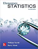
The relationship between inflation and unemployment is not very strong. However .if we are interested in predicting unemployment, we would probably want to predict next year’s unemployment from this year’s inflation we can construct equation to do this by matching each year? Inflation with the next year’s unemployment. As shown in the following table.
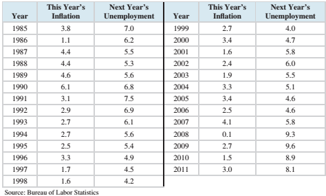
Compute the least-squares line for predicting next year’s unemployment from this year’s inflation
To calculate:
To compute the least squares regression line for the given data set.
Answer to Problem 6CS
Explanation of Solution
Given information:
The following table presents the inflation rate and unemployment rate, both in percent, for the years 1985-2012.
| Year | Inflation | Unemployment |
| 1985 | 3.8 | 7.0 |
| 1986 | 1.1 | 6.2 |
| 1987 | 4.4 | 5.5 |
| 1988 | 4.4 | 5.3 |
| 1989 | 4.6 | 5.6 |
| 1990 | 6.1 | 6.8 |
| 1991 | 3.1 | 7.5 |
| 1992 | 2.9 | 6.9 |
| 1993 | 2.7 | 6.1 |
| 1994 | 2.7 | 5.6 |
| 1995 | 2.5 | 5.4 |
| 1996 | 3.3 | 4.9 |
| 1997 | 1.7 | 4.5 |
| 1998 | 1.6 | 4.2 |
| 1999 | 2.7 | 4.0 |
| 2000 | 3.4 | 4.7 |
| 2001 | 1.6 | 5.8 |
| 2002 | 2.4 | 6.0 |
| 2003 | 1.9 | 5.5 |
| 2004 | 3.3 | 5.1 |
| 2005 | 3.4 | 4.6 |
| 2006 | 2.5 | 4.6 |
| 2007 | 4.1 | 5.8 |
| 2008 | 0.1 | 9.3 |
| 2009 | 2.7 | 9.6 |
| 2010 | 1.5 | 8.9 |
| 2011 | 3.0 | 8.1 |
Formula Used:
The equation for least-square regression line:
Where
The correlation coefficient of a data is given by:
Where,
The standard deviations are given by:
The mean of x is given by:
The mean of y is given by:
Calculation:
The mean of x is given by:
The mean of y is given by:
The data can be represented in tabular form as:
| x | y |  |
 |
 |
 |
| 3.8 | 7.0 | 0.92963 | 0.86421 | 0.94444 | 0.89198 |
| 1.1 | 6.2 | -1.77037 | 3.13421 | 0.14444 | 0.02086 |
| 4.4 | 5.5 | 1.52963 | 2.33977 | -0.55556 | 0.30864 |
| 4.4 | 5.3 | 1.52963 | 2.33977 | -0.75556 | 0.57086 |
| 4.6 | 5.6 | 1.72963 | 2.99162 | -0.45556 | 0.20753 |
| 6.1 | 6.8 | 3.22963 | 10.43051 | 0.74444 | 0.55420 |
| 3.1 | 7.5 | 0.22963 | 0.05273 | 1.44444 | 2.08642 |
| 2.9 | 6.9 | 0.02963 | 0.00088 | 0.84444 | 0.71309 |
| 2.7 | 6.1 | -0.17037 | 0.02903 | 0.04444 | 0.00198 |
| 2.7 | 5.6 | -0.17037 | 0.02903 | -0.45556 | 0.20753 |
| 2.5 | 5.4 | -0.37037 | 0.13717 | -0.65556 | 0.42975 |
| 3.3 | 4.9 | 0.42963 | 0.18458 | -1.15556 | 1.33531 |
| 1.7 | 4.5 | -1.17037 | 1.36977 | -1.55556 | 2.41975 |
| 1.6 | 4.2 | -1.27037 | 1.61384 | -1.85556 | 3.44309 |
| 2.7 | 4.0 | -0.17037 | 0.02903 | -2.05556 | 4.22531 |
| 3.4 | 4.7 | 0.52963 | 0.28051 | -1.35556 | 1.83753 |
| 1.6 | 5.8 | -1.27037 | 1.61384 | -0.25556 | 0.06531 |
| 2.4 | 6.0 | -0.47037 | 0.22125 | -0.05556 | 0.00309 |
| 1.9 | 5.5 | -0.97037 | 0.94162 | -0.55556 | 0.30864 |
| 3.3 | 5.1 | 0.42963 | 0.18458 | -0.95556 | 0.91309 |
| 3.4 | 4.6 | 0.52963 | 0.28051 | -1.45556 | 2.11864 |
| 2.5 | 4.6 | -0.37037 | 0.13717 | -1.45556 | 2.11864 |
| 4.1 | 5.8 | 1.22963 | 1.51199 | -0.25556 | 0.06531 |
| 0.1 | 9.3 | -2.77037 | 7.67495 | 3.24444 | 10.52642 |
| 2.7 | 9.6 | -0.17037 | 0.02903 | 3.54444 | 12.56309 |
| 1.5 | 8.9 | -1.37037 | 1.87791 | 2.84444 | 8.09086 |
| 3.0 | 8.1 | 0.12963 | 0.01680 | 2.04444 | 4.17975 |
| |
|
|
|
Hence, the standard deviation is given by:
And,
Consider,
Hence, the table for calculating coefficient of correlation is given by:
| x | y |  |
 |
 |
| 3.8 | 7.0 | 0.92963 | 0.94444 | 0.87798 |
| 1.1 | 6.2 | -1.77037 | 0.14444 | -0.25572 |
| 4.4 | 5.5 | 1.52963 | -0.55556 | -0.84979 |
| 4.4 | 5.3 | 1.52963 | -0.75556 | -1.15572 |
| 4.6 | 5.6 | 1.72963 | -0.45556 | -0.78794 |
| 6.1 | 6.8 | 3.22963 | 0.74444 | 2.40428 |
| 3.1 | 7.5 | 0.22963 | 1.44444 | 0.33169 |
| 2.9 | 6.9 | 0.02963 | 0.84444 | 0.02502 |
| 2.7 | 6.1 | -0.17037 | 0.04444 | -0.00757 |
| 2.7 | 5.6 | -0.17037 | -0.45556 | 0.07761 |
| 2.5 | 5.4 | -0.37037 | -0.65556 | 0.24280 |
| 3.3 | 4.9 | 0.42963 | -1.15556 | -0.49646 |
| 1.7 | 4.5 | -1.17037 | -1.55556 | 1.82058 |
| 1.6 | 4.2 | -1.27037 | -1.85556 | 2.35724 |
| 2.7 | 4.0 | -0.17037 | -2.05556 | 0.35021 |
| 3.4 | 4.7 | 0.52963 | -1.35556 | -0.71794 |
| 1.6 | 5.8 | -1.27037 | -0.25556 | 0.32465 |
| 2.4 | 6.0 | -0.47037 | -0.05556 | 0.02613 |
| 1.9 | 5.5 | -0.97037 | -0.55556 | 0.53909 |
| 3.3 | 5.1 | 0.42963 | -0.95556 | -0.41053 |
| 3.4 | 4.6 | 0.52963 | -1.45556 | -0.77091 |
| 2.5 | 4.6 | -0.37037 | -1.45556 | 0.53909 |
| 4.1 | 5.8 | 1.22963 | -0.25556 | -0.31424 |
| 0.1 | 9.3 | -2.77037 | 3.24444 | -8.98831 |
| 2.7 | 9.6 | -0.17037 | 3.54444 | -0.60387 |
| 1.5 | 8.9 | -1.37037 | 2.84444 | -3.89794 |
| 3.0 | 8.1 | 0.12963 | 2.04444 | 0.26502 |
| |
|
|
Plugging the values in the formula,
Plugging the values to obtain b1,
Plugging the values to obtain b0,
Hence, the least-square regression line is given by:
Therefore, the least squares regression line for the given data set is
Want to see more full solutions like this?
Chapter 4 Solutions
Elementary Statistics 2nd Edition


 Calculus For The Life SciencesCalculusISBN:9780321964038Author:GREENWELL, Raymond N., RITCHEY, Nathan P., Lial, Margaret L.Publisher:Pearson Addison Wesley,
 Linear Algebra: A Modern IntroductionAlgebraISBN:9781285463247Author:David PoolePublisher:Cengage Learning
 Trigonometry (MindTap Course List)TrigonometryISBN:9781305652224Author:Charles P. McKeague, Mark D. TurnerPublisher:Cengage Learning
 Algebra & Trigonometry with Analytic GeometryAlgebraISBN:9781133382119Author:SwokowskiPublisher:Cengage