
Concept explainers
Videos
The following table, Reproduce from chapter introduction. Presents the inflation rate and unemployment rate, both in percent, for the years 1985-2012
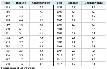
We will investigate some methods for predicting unemployment first. We will try to predict the unemployment rate from the inflation rate.
Compute the least-squares line for predicting unemployment from inflation.
To calculate: To compute the least squares regression line for the given data set.
Answer to Problem 2CS
Explanation of Solution
Given information:
The following table presents the inflation rate and unemployment rate, both in percent, for the years 1985-2012.
| Year | Inflation | Unemployment |
| 1985 | 3.8 | 7.2 |
| 1986 | 1.1 | 7.0 |
| 1987 | 4.4 | 6.2 |
| 1988 | 4.4 | 5.5 |
| 1989 | 4.6 | 5.3 |
| 1990 | 6.1 | 5.6 |
| 1991 | 3.1 | 6.8 |
| 1992 | 2.9 | 7.5 |
| 1993 | 2.7 | 6.9 |
| 1994 | 2.7 | 6.1 |
| 1995 | 2.5 | 5.6 |
| 1996 | 3.3 | 5.4 |
| 1997 | 1.7 | 4.9 |
| 1998 | 1.6 | 4.5 |
| 1999 | 2.7 | 4.2 |
| 2000 | 3.4 | 4.0 |
| 2001 | 1.6 | 4.7 |
| 2002 | 2.4 | 5.8 |
| 2003 | 1.9 | 6.0 |
| 2004 | 3.3 | 5.5 |
| 2005 | 3.4 | 5.1 |
| 2006 | 2.5 | 4.6 |
| 2007 | 4.1 | 4.6 |
| 2008 | 0.1 | 5.8 |
| 2009 | 2.7 | 9.3 |
| 2010 | 1.5 | 9.6 |
| 2011 | 3.0 | 8.9 |
| 2012 | 1.7 | 8.1 |
Formula Used:
The equation for least-square regression line:
Where
The correlation coefficient of a data is given by:
Where,
The standard deviations are given by:
The mean of x is given by:
The mean of y is given by:
Calculation:
The mean of x is given by:
The mean of y is given by:
The data can be represented in tabular form as:
| x | y |  |  |  |  |
| 3.8 | 7.2 | 0.97143 | 0.94367 | 1.10357 | 1.21787 |
| 1.1 | 7.0 | -1.72857 | 2.98796 | 0.90357 | 0.81644 |
| 4.4 | 6.2 | 1.57143 | 2.46939 | 0.10357 | 0.01073 |
| 4.4 | 5.5 | 1.57143 | 2.46939 | -0.59643 | 0.35573 |
| 4.6 | 5.3 | 1.77143 | 3.13796 | -0.79643 | 0.63430 |
| 6.1 | 5.6 | 3.27143 | 10.70224 | -0.49643 | 0.24644 |
| 3.1 | 6.8 | 0.27143 | 0.07367 | 0.70357 | 0.49501 |
| 2.9 | 7.5 | 0.07143 | 0.00510 | 1.40357 | 1.97001 |
| 2.7 | 6.9 | -0.12857 | 0.01653 | 0.80357 | 0.64573 |
| 2.7 | 6.1 | -0.12857 | 0.01653 | 0.00357 | 0.00001 |
| 2.5 | 5.6 | -0.32857 | 0.10796 | -0.49643 | 0.24644 |
| 3.3 | 5.4 | 0.47143 | 0.22224 | -0.69643 | 0.48501 |
| 1.7 | 4.9 | -1.12857 | 1.27367 | -1.19643 | 1.43144 |
| 1.6 | 4.5 | -1.22857 | 1.50939 | -1.59643 | 2.54858 |
| 2.7 | 4.2 | -0.12857 | 0.01653 | -1.89643 | 3.59644 |
| 3.4 | 4.0 | 0.57143 | 0.32653 | -2.09643 | 4.39501 |
| 1.6 | 4.7 | -1.22857 | 1.50939 | -1.39643 | 1.95001 |
| 2.4 | 5.8 | -0.42857 | 0.18367 | -0.29643 | 0.08787 |
| 1.9 | 6.0 | -0.92857 | 0.86224 | -0.09643 | 0.00930 |
| 3.3 | 5.5 | 0.47143 | 0.22224 | -0.59643 | 0.35573 |
| 3.4 | 5.1 | 0.57143 | 0.32653 | -0.99643 | 0.99287 |
| 2.5 | 4.6 | -0.32857 | 0.10796 | -1.49643 | 2.23930 |
| 4.1 | 4.6 | 1.27143 | 1.61653 | -1.49643 | 2.23930 |
| 0.1 | 5.8 | -2.72857 | 7.44510 | -0.29643 | 0.08787 |
| 2.7 | 9.3 | -0.12857 | 0.01653 | 3.20357 | 10.26287 |
| 1.5 | 9.6 | -1.32857 | 1.76510 | 3.50357 | 12.27501 |
| 3.0 | 8.9 | 0.17143 | 0.02939 | 2.80357 | 7.86001 |
| 1.7 | 8.1 | -1.12857 | 1.27367 | 2.00357 | 4.01430 |
Hence, the standard deviation is given by:
And,
Consider,
Hence, the table for calculating coefficient of correlation is given by:
| x | y |  |  |  |
| 3.8 | 7.2 | 0.97143 | 1.10357 | 1.07204 |
| 1.1 | 7.0 | -1.72857 | 0.90357 | -1.56189 |
| 4.4 | 6.2 | 1.57143 | 0.10357 | 0.16276 |
| 4.4 | 5.5 | 1.57143 | -0.59643 | -0.93724 |
| 4.6 | 5.3 | 1.77143 | -0.79643 | -1.41082 |
| 6.1 | 5.6 | 3.27143 | -0.49643 | -1.62403 |
| 3.1 | 6.8 | 0.27143 | 0.70357 | 0.19097 |
| 2.9 | 7.5 | 0.07143 | 1.40357 | 0.10026 |
| 2.7 | 6.9 | -0.12857 | 0.80357 | -0.10332 |
| 2.7 | 6.1 | -0.12857 | 0.00357 | -0.00046 |
| 2.5 | 5.6 | -0.32857 | -0.49643 | 0.16311 |
| 3.3 | 5.4 | 0.47143 | -0.69643 | -0.32832 |
| 1.7 | 4.9 | -1.12857 | -1.19643 | 1.35026 |
| 1.6 | 4.5 | -1.22857 | -1.59643 | 1.96133 |
| 2.7 | 4.2 | -0.12857 | -1.89643 | 0.24383 |
| 3.4 | 4.0 | 0.57143 | -2.09643 | -1.19796 |
| 1.6 | 4.7 | -1.22857 | -1.39643 | 1.71561 |
| 2.4 | 5.8 | -0.42857 | -0.29643 | 0.12704 |
| 1.9 | 6.0 | -0.92857 | -0.09643 | 0.08954 |
| 3.3 | 5.5 | 0.47143 | -0.59643 | -0.28117 |
| 3.4 | 5.1 | 0.57143 | -0.99643 | -0.56939 |
| 2.5 | 4.6 | -0.32857 | -1.49643 | 0.49168 |
| 4.1 | 4.6 | 1.27143 | -1.49643 | -1.90260 |
| 0.1 | 5.8 | -2.72857 | -0.29643 | 0.80883 |
| 2.7 | 9.3 | -0.12857 | 3.20357 | -0.41189 |
| 1.5 | 9.6 | -1.32857 | 3.50357 | -4.65474 |
| 3.0 | 8.9 | 0.17143 | 2.80357 | 0.48061 |
| 1.7 | 8.1 | -1.12857 | 2.00357 | -2.26117 |
Plugging the values in the formula,
Plugging the values to obtain b1 ,
Plugging the values to obtain b0 ,
Hence, the least-square regression line is given by:
Therefore, the least squares regression line for the given data set is
Want to see more full solutions like this?
Chapter 4 Solutions
Elementary Statistics 2nd Edition


- Table 2 shows a recent graduate’s credit card balance each month after graduation. a. Use exponential regression to fit a model to these data. b. If spending continues at this rate, what will the graduate’s credit card debt be one year after graduating?arrow_forwardTable 6 shows the population, in thousands, of harbor seals in the Wadden Sea over the years 1997 to 2012. a. Let x represent time in years starting with x=0 for the year 1997. Let y represent the number of seals in thousands. Use logistic regression to fit a model to these data. b. Use the model to predict the seal population for the year 2020. c. To the nearest whole number, what is the limiting value of this model?arrow_forwardDoes Table 1 represent a linear function? If so, finda linear equation that models the data.arrow_forward
 Calculus For The Life SciencesCalculusISBN:9780321964038Author:GREENWELL, Raymond N., RITCHEY, Nathan P., Lial, Margaret L.Publisher:Pearson Addison Wesley,
 Algebra & Trigonometry with Analytic GeometryAlgebraISBN:9781133382119Author:SwokowskiPublisher:Cengage
 Linear Algebra: A Modern IntroductionAlgebraISBN:9781285463247Author:David PoolePublisher:Cengage Learning
 Trigonometry (MindTap Course List)TrigonometryISBN:9781305652224Author:Charles P. McKeague, Mark D. TurnerPublisher:Cengage Learning
 Algebra and Trigonometry (MindTap Course List)AlgebraISBN:9781305071742Author:James Stewart, Lothar Redlin, Saleem WatsonPublisher:Cengage Learning