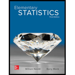
Elementary Statistics ( 3rd International Edition ) Isbn:9781260092561
3rd Edition
ISBN: 9781259969454
Author: William Navidi Prof.; Barry Monk Professor
Publisher: McGraw-Hill Education
expand_more
expand_more
format_list_bulleted
Concept explainers
Question
Chapter 4, Problem 6CQ
To determine
To find the least square regression line for the given data
Expert Solution & Answer
Want to see the full answer?
Check out a sample textbook solution
Students have asked these similar questions
explain the importance of the Hypothesis test in a business setting, and give an example of a situation where it is helpful in business decision making.
A college wants to estimate what students typically spend on textbooks. A report fromthe college bookstore observes that textbooks range in price from $22 to $186. Toobtain a 95% confidence level for a confidence interval estimate to plus or minus $10,how many students should the college survey? (We may estimate the populationstandard deviation as (range) ÷ 4.)
In a study of how students give directions, forty volunteers were given the task ofexplaining to another person how to reach a destination. Researchers measured thefollowing five aspects of the subjects’ direction-giving behavior:• whether a map was available or if directions were given from memory without a map,• the gender of the direction-giver,• the distances given as part of the directions,• the number of times directions such as “north” or “left” were used,• the frequency of errors in directions.
Identify each of the variables in this study, and whether each is quantitative orqualitative. For each quantitative variable, state whether it is discrete or continuous.
Was this an observational study or an experimental study? Explain your answer.
Chapter 4 Solutions
Elementary Statistics ( 3rd International Edition ) Isbn:9781260092561
Ch. 4.1 - In Exercises 9-12, fill in each blank with the...Ch. 4.1 - In Exercises 9-12, fill in each blank with the...Ch. 4.1 - In Exercises 9-12, fill in each blank with the...Ch. 4.1 - In Exercises 9-12, fill in each blank with the...Ch. 4.1 - Prob. 13ECh. 4.1 - Prob. 14ECh. 4.1 - In Exercises 13-16, determine whether the...Ch. 4.1 - In Exercises 13-16, determine whether the...Ch. 4.1 - In Exercises 17-20, compute the correlation...Ch. 4.1 - In Exercises 17-20, compute the correlation...
Ch. 4.1 - In Exercises 17-20, compute the correlation...Ch. 4.1 - In Exercises 17-20, compute the correlation...Ch. 4.1 - In Exercises 21-24, determine whether the...Ch. 4.1 - In Exercises 21-24, determine whether the...Ch. 4.1 - In Exercises 21-24, determine whether the...Ch. 4.1 - In Exercises 21-24, determine whether the...Ch. 4.1 - In Exercises 25-30, determine whether the...Ch. 4.1 - In Exercises 25-30, determine whether the...Ch. 4.1 - In Exercises 25-30, determine whether the...Ch. 4.1 - In Exercises 25-30, determine whether the...Ch. 4.1 - In Exercises 25-30, determine whether the...Ch. 4.1 - In Exercises 25-30, determine whether the...Ch. 4.1 - Price of eggs and milk: The following table...Ch. 4.1 - Government funding: The following table presents...Ch. 4.1 - Pass the ball: The following table lists the...Ch. 4.1 - Carbon footprint: Carbon dioxide (CO2) is produced...Ch. 4.1 - Foot temperatures: Foot ulcers are a common...Ch. 4.1 - Mortgage payments: The following table presents...Ch. 4.1 - Blood pressure: A blood pressure measurement...Ch. 4.1 - Prob. 38ECh. 4.1 - Police and crime: In a survey of cities in the...Ch. 4.1 - Age and education: A survey of U.S. adults showed...Ch. 4.1 - Whats the correlation? In a sample of adults, the...Ch. 4.1 - Prob. 42ECh. 4.1 - Changing means and standard deviations: A small...Ch. 4.2 - In Exercises 5-7, fill in each blank with the...Ch. 4.2 - In Exercises 5-7, fill in each blank with the...Ch. 4.2 - In Exercises 5-7, fill in each blank with the...Ch. 4.2 - Prob. 8ECh. 4.2 - Prob. 9ECh. 4.2 - Prob. 10ECh. 4.2 - Prob. 11ECh. 4.2 - Prob. 12ECh. 4.2 - In Exercises 13-16, compute the least-squares...Ch. 4.2 - In Exercises 13-16, compute the least-squares...Ch. 4.2 - In Exercises 13-16, compute the least-squares...Ch. 4.2 - In Exercises 13-16, compute the least-squares...Ch. 4.2 - Compute the least-squares regression he for...Ch. 4.2 - Compute the least-squares regression he for...Ch. 4.2 - In a hypothetical study of the relationship...Ch. 4.2 - Assume in a study of educational level in years...Ch. 4.2 - Price of eggs and milk: The following table...Ch. 4.2 - Government funding: The following table presents...Ch. 4.2 - Pass the ball: The following table lists the...Ch. 4.2 - Carbon footprint: Carbon dioxide (CO2) is produced...Ch. 4.2 - Foot temperatures: Foot ulcers are a common...Ch. 4.2 - Mortgage payments: The following table presents...Ch. 4.2 - Blood pressure: A blood pressure measurement...Ch. 4.2 - Butterfly wings: Do larger butterflies live...Ch. 4.2 - Interpreting technology: The following display...Ch. 4.2 - Interpreting technology: The following display...Ch. 4.2 - Interpreting technology: The following MINITAB...Ch. 4.2 - Interpreting technology: The following MINITAB...Ch. 4.2 - Prob. 33ECh. 4.2 - Prob. 34ECh. 4.2 - Least-squares regression line for z-scores: The...Ch. 4.3 - In Exercises 5-10, fill in each blank with the...Ch. 4.3 - In Exercises 5-10, fill in each blank with the...Ch. 4.3 - In Exercises 5-10, fill in each blank with the...Ch. 4.3 - In Exercises 5-10, fill in each blank with the...Ch. 4.3 - In Exercises 5-10, fill in each blank with the...Ch. 4.3 - Prob. 10ECh. 4.3 - Prob. 11ECh. 4.3 - In Exercises 11-14, determine whether the...Ch. 4.3 - Prob. 13ECh. 4.3 - In Exercises 11-14, determine whether the...Ch. 4.3 - For the following data set: Compute the...Ch. 4.3 - For the following data set: Compute the...Ch. 4.3 - For the following data set: Compute the...Ch. 4.3 - For the following data set: Compute the...Ch. 4.3 - Prob. 19ECh. 4.3 - Prob. 20ECh. 4.3 - Prob. 21ECh. 4.3 - Prob. 22ECh. 4.3 - Hot enough for you? The following table presents...Ch. 4.3 - Presidents and first ladies: The presents the ages...Ch. 4.3 - Mutant genes: In a study to determine whether the...Ch. 4.3 - Imports and exports: The following table presents...Ch. 4.3 - Energy consumption: The following table presents...Ch. 4.3 - Cost of health care: The following table presents...Ch. 4.3 - Prob. 29ECh. 4.3 - Prob. 30ECh. 4.3 - Prob. 31ECh. 4.3 - Transforming a variable: The following table...Ch. 4.3 - Prob. 33ECh. 4.3 - Prob. 34ECh. 4 - Compute the correlation coefficient for the...Ch. 4 - The number of theaters showing the movie Monsters...Ch. 4 - Use the data in Exercise 2 to compute the...Ch. 4 - A scatterplot has a correlation of r=1. Describe...Ch. 4 - Prob. 5CQCh. 4 - Prob. 6CQCh. 4 - Use the least-squares regression line computed in...Ch. 4 - Use the least-squares regression line computed in...Ch. 4 - Prob. 9CQCh. 4 - A scatterplot has a least-squares regression line...Ch. 4 - Prob. 11CQCh. 4 - Prob. 12CQCh. 4 - A sample of students was studied to determine the...Ch. 4 - In a scatter-plot; the point (-2, 7) is...Ch. 4 - The correlation coefficient for a data set is...Ch. 4 - Prob. 1RECh. 4 - Prob. 2RECh. 4 - Hows your mileage? Weight (in tons) and fuel...Ch. 4 - Prob. 4RECh. 4 - Energy efficiency: A sample of 10 households was...Ch. 4 - Energy efficiency: Using the data in Exercise 5:...Ch. 4 - Prob. 7RECh. 4 - Prob. 8RECh. 4 - Prob. 9RECh. 4 - Prob. 10RECh. 4 - Baby weights: The average gestational age (time...Ch. 4 - Commute times: Every morning, Tania leaves for...Ch. 4 - Prob. 13RECh. 4 - Prob. 14RECh. 4 - Prob. 15RECh. 4 - Describe an example which two variables are...Ch. 4 - Two variables x and y have a positive association...Ch. 4 - Prob. 3WAICh. 4 - Prob. 4WAICh. 4 - Prob. 5WAICh. 4 - Prob. 6WAICh. 4 - Prob. 7WAICh. 4 - Prob. 8WAICh. 4 - Prob. 9WAICh. 4 - The following table, reproduced from the chapter...Ch. 4 - Prob. 2CSCh. 4 - Prob. 3CSCh. 4 - Prob. 4CSCh. 4 - Prob. 5CSCh. 4 - Prob. 6CSCh. 4 - Prob. 7CSCh. 4 - Prob. 8CSCh. 4 - Prob. 9CSCh. 4 - Prob. 10CSCh. 4 - Prob. 11CSCh. 4 - Prob. 12CSCh. 4 - Prob. 13CSCh. 4 - If we are going to use data from this year to...Ch. 4 - Prob. 15CS
Knowledge Booster
Learn more about
Need a deep-dive on the concept behind this application? Look no further. Learn more about this topic, statistics and related others by exploring similar questions and additional content below.Similar questions
- explain the difference between the confident interval and the confident level. provide an example to show how to correctly interpret a confidence interval.arrow_forwardSketch to scale the orbit of Earth about the sun. Graph Icarus’ orbit on the same set of axesWhile the sun is the center of Earth’s orbit, it is a focus of Icarus’ orbit. There aretwo points of intersection on the graph. Based on the graph, what is the approximate distance between the two points of intersection (in AU)?arrow_forwardThe diameters of ball bearings are distributed normally. The mean diameter is 67 millimeters and the standard deviation is 3 millimeters. Find the probability that the diameter of a selected bearing is greater than 63 millimeters. Round to four decimal places.arrow_forward
- Suppose you like to keep a jar of change on your desk. Currently, the jar contains the following: 22 Pennies 27 Dimes 9 Nickels 30 Quarters What is the probability that you reach into the jar and randomly grab a penny and then, without replacement, a dime? Express as a fraction or a decimal number rounded to four decimal places.arrow_forwardA box contains 14 large marbles and 10 small marbles. Each marble is either green or white. 9 of the large marbles are green, and 4 of the small marbles are white. If a marble is randomly selected from the box, what is the probability that it is small or white? Express as a fraction or a decimal number rounded to four decimal places.arrow_forwardCan I get help with this step please? At a shooting range, instructors can determine if a shooter is consistently missing the target because of the gun sight or because of the shooter's ability. If a gun's sight is off, the variance of the distances between the shots and the center of the shot pattern will be small (even if the shots are not in the center of the target). A student claims that it is the sight that is off, not his aim, and wants the instructor to confirm his claim. If a skilled shooter fires a gun at a target multiple times, the distances between the shots and the center of the shot pattern, measured in centimeters (cm), will have a variance of less than 0.33. After the student shoots 28 shots at the target, the instructor calculates that the distances between his shots and the center of the shot pattern, measured in cm, have a variance of 0.25. Does this evidence support the student's claim that the gun's sight is off? Use a 0.025 level of significance. Assume that the…arrow_forward
- The National Academy of Science reported that 38% of research in mathematics is published by US authors. The mathematics chairperson of a prestigious university wishes to test the claim that this percentage is no longer 38%. He has no indication of whether the percentage has increased or decreased since that time. He surveys a simple random sample of 279 recent articles published by reputable mathematics research journals and finds that 123 of these articles have US authors. Does this evidence support the mathematics chairperson's claim that the percentage is no longer 38 % ? Use a 0.02 level of significance. Compute the value of the test statistic. Round to two decimal places.arrow_forwardA marketing research company desires to know the mean consumption of milk per week among males over age 32. They believe that the milk consumption has a mean of 4 liters, and want to construct a 98% confidence interval with a maximum error of 0.07 liters. Assuming a variance of 0.64 liters, what is the minimum number of males over age 32 they must include in their sample? Round up to the next integer.arrow_forwardSuppose GRE Verbal scores are normally distributed with a mean of 461 and a standard deviation of 118. A university plans to recruit students whose scores are in the top 4 % . What is the minimum score required for recruitment? Round to the nearest whole number, if necessaryarrow_forward
- Need help with my homework thank you random sample of 6 fields of durum wheat has a mean yield of 45.5 bushels per acre and standard deviation of 7.43 bushels per acre. Determine the 80 % confidence interval for the true mean yield. Assume the population is approximately normal. Step 1: Find the critical value that should be used in constructing the confidence interval. Round to three decimal places. Step 2 of 2: Construct the 80% confidence interval. Round to one decimal place. I got 1.476 as my critical value and 41.0 and 49.9 as my confidence intervalarrow_forwardCan someone check my work? If you draw a card with a value of four or less from a standard deck of cards, I will pay you $14. If not, you pay me $8. (Aces are considered the highest card in the deck.) Step 1 of 2: Find the expected value of the proposition. Round to two decimal places. Losses must be expressed as negative values. PT 2: If you played this game 718 times how much would you expect to win or lose? Round your answer to two decimal places. Losses must be expressed as negative values. for part 1 I got -2.92 pt 2 -2097.56arrow_forwardThe following table describes the distribution of a random sample S of 200 individuals, arranged by education level and income. Income(Dollars per Year) < High School High School Diploma Some College Bachelor’s Degree Graduate Degree Post-Graduate Degree 0-25,000 12 8 3 2 1 0 25,000-50,000 7 12 9 12 11 2 50,000-75,000 1 3 4 6 14 5 75,000-100,000 0 2 1 8 11 8 100,000-125,000 0 1 1 4 8 9 125,000-150,000 0 0 2 3 7 12 150,000+ 0 0 1 1 3 6 Let events be defined as follows: A = the event the subject makes 0-25,000 dollars per yearB = the event the subject makes 25,000-50,000 dollars per year C = the event the subject makes 50,000-75,000 dollars per yearD = the event the subject makes 75,000-100,000 dollars per yearE = the event the subject makes 100,000-125,000 dollars per yearF = the event the subject makes 125,000-150,000 dollars per yearG = the event…arrow_forward
arrow_back_ios
SEE MORE QUESTIONS
arrow_forward_ios
Recommended textbooks for you
 Linear Algebra: A Modern IntroductionAlgebraISBN:9781285463247Author:David PoolePublisher:Cengage Learning
 Elementary Linear Algebra (MindTap Course List)AlgebraISBN:9781305658004Author:Ron LarsonPublisher:Cengage Learning
 Big Ideas Math A Bridge To Success Algebra 1: Stu...AlgebraISBN:9781680331141Author:HOUGHTON MIFFLIN HARCOURTPublisher:Houghton Mifflin Harcourt
 Glencoe Algebra 1, Student Edition, 9780079039897...AlgebraISBN:9780079039897Author:CarterPublisher:McGraw Hill
 College AlgebraAlgebraISBN:9781305115545Author:James Stewart, Lothar Redlin, Saleem WatsonPublisher:Cengage Learning

Linear Algebra: A Modern Introduction
Algebra
ISBN:9781285463247
Author:David Poole
Publisher:Cengage Learning

Elementary Linear Algebra (MindTap Course List)
Algebra
ISBN:9781305658004
Author:Ron Larson
Publisher:Cengage Learning

Big Ideas Math A Bridge To Success Algebra 1: Stu...
Algebra
ISBN:9781680331141
Author:HOUGHTON MIFFLIN HARCOURT
Publisher:Houghton Mifflin Harcourt

Glencoe Algebra 1, Student Edition, 9780079039897...
Algebra
ISBN:9780079039897
Author:Carter
Publisher:McGraw Hill


College Algebra
Algebra
ISBN:9781305115545
Author:James Stewart, Lothar Redlin, Saleem Watson
Publisher:Cengage Learning
Correlation Vs Regression: Difference Between them with definition & Comparison Chart; Author: Key Differences;https://www.youtube.com/watch?v=Ou2QGSJVd0U;License: Standard YouTube License, CC-BY
Correlation and Regression: Concepts with Illustrative examples; Author: LEARN & APPLY : Lean and Six Sigma;https://www.youtube.com/watch?v=xTpHD5WLuoA;License: Standard YouTube License, CC-BY