
Subpart (a):
The consumer surplus , total surplus and deadweight loss .
Subpart (a):
Explanation of Solution
Figure -1 illustrates the
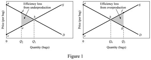
In figure -1 panel (a) and (b), the horizontal axis measures the quantity of bags and the vertical axis measures the price per bag. The curve ‘S’ represents the supply and the curve ‘D’ represents the demand.
The inverse demand function can be derived as follows:
The inverse demand functions of
The inverse supply curve can be calculated as follows:
The inverse supply functions of
The inverse demand function and supply functions reveal that the producer willing price is $5 and the consumer willing price is $85. The equilibrium price is $45. The total surplus can be calculated as follows:
The total surplus is $800.
The consumer surplus can be calculated as follows:
The consumer surplus is $400.
Concept Introduction:
Consumer surplus: It refers to the variation in the probable charge of a product that the consumer intends to pay and the actual price that he has already paid.
Subpart (b):
The consumer surplus, total surplus and deadweight loss.
Subpart (b):
Explanation of Solution
The consumer willing price at Q2 level of output (15 units) can be calculated by substituting the Q2 level of output to the inverse demand function.
The consumer new willing price is $55.
The producer willing price at Q2 level of output (15 units) can be calculated by substituting the Q2 level of output into the inverse supply function.
The producer’s new willing price is $35.
The deadweight loss can be calculated as follows:
The deadweight loss is $50.
The total surplus can be calculated as follows:
The total surplus is $750.
Concept Introduction:
Consumer surplus: It refers to the variation in the probable charge of a product that the consumer intends to pay and the actual price that he has already paid.
Producer surplus: It refers to the variation in the probable price that the producer intends to sell and the actual price that he has already sold.
Subpart c):
The consumer surplus, total surplus and deadweight loss.
Subpart c):
Explanation of Solution
The consumer willing price at Q3 level of output (27 units) can be calculated by substituting the Q3 level of output to the inverse demand function.
The consumer new willing price is $31.
The producer willing price at Q3 level of output (127 units) can be calculated by substituting the Q3 level of output to the inverse supply function.
The producer new willing price is $59.
The deadweight loss can be calculated as follows:
The deadweight loss is $98.
The total surplus can be calculated as follows:
The total surplus is $702.
Concept Introduction:
Consumer surplus: It refers to the variation in the probable charge of a product that the consumer intends to pay and the actual price that he has already paid.
Producer surplus: It refers to the variation in the probable price that the producer intends to sell and the actual price that he has already sold.
Want to see more full solutions like this?
Chapter 4 Solutions
Gen Combo Microeconomics; Connect Access Card

- For all questions, refer to the graph on the reverse side. Use this graph for 1 – 4. The graph represents the market for coffee. Estimation may be necessary, so show work. Name a good that will see increased sales due to the tariff or quota above. Name a good besides coffee that will see decreased sales due to the tariff or quota above. Suppose that 1 US$ = 1.5 South African Rand. Also, suppose that the representative good, peanut butter, is $3 per jar in the US and 4 Rand per jar in SA. How will this situation affect the exchange market for U.S. dollars? Explain/show the effect(s) of these prices. Include the initial effect(s), the market adjustment(s), and the final result(s) on equilibrium.arrow_forwardWhen filing an income tax return, one can claim a deduction for charitable contributions. Let's simplify the income tax system and assume that the tax is proportional to the level of taxable income (income after deductions). (a) Suppose we increase the marginal income tax rate. An economic adviser claims that the effect of this tax change on the amount of charitable contributions is uncertain. Plot a simple graph that illustrates this situation (it involves the choice between charitable contributions and other spending), use it to explain why the effect is uncertain and explain what it depends on. (b) Now suppose that we instead increase the marginal tax rate but also provide a transfer that makes the bundle that used to be optimal before tax increased just affordable. According to the economic adviser this policy change will make people contribute more to charity. Why?arrow_forwardNow assume we can derive an economic analysis from the biological relationship. Fisherman select the number of boats to operate - boats will be the choice of EFFORT. Boats Total Harvest 0 (tons) 0 100 200 300 400 500 600 700 800 900 1,200 2,200 2,800 3,000 2,800 2,400 1,600 800 Suppose the price of fish is $1,000 per ton. Suppose the cost to operate a boat for a year is $4,000. Construct a graph showing the total revenue and cost of the fishery. 0 What is the highest profit that can be earned, and how many boats are used for this? ( What is the corresponding long-run stock level associated with the profit-maximizing choice of effort? What is the profit earned if fisherman harvested the MSY? What number of boats are used in open access?arrow_forward
- K possible A A small town provides a fireworks display, which is a public good, every fourth of July. For simplicity, assume the town only has two residents: Hayden and Madison. Their demands for the fireworks display are illustrated in the figure to the right. Construct the market demand curve for this public good. Use the line drawing tool to draw the market demand curve (DMarket) for the fireworks display. Properly label this line. Carefully follow the instructions above, and only draw the required objects. Price (dollars per firework) 8.00T 7.50- 7.00- C 6.50- 6.00- 5.50- 5.00- 4.50- 4.00- 3.50- Madison Hayden 3.00- 2.50- 2.00- 1.50 1.00- 0.50- 0.00 0 2 4 6 8 10 12 14 1 Quantity (number of fireworks)arrow_forward1.) Use the line drawing tool to draw the equation Y = 1 + 1.50X. Label your line 'A'. 20- 2.) Use the line drawing tool to draw the equation Y = 18 – 1.50X. Label your line 18- 'B'. 16- 3.) Use the point drawing tool to indicate the point where both equations are equal. Label this point 'Equilibrium'. 14- Carefully follow the instructions above, and only draw the required objects. g 12- 10- 8- 6- 4- 2- 0- 4 6. 8 10 12 14 16 18 20 Quantity (Q) Price P = f(Q) -coarrow_forward7 (a) Assume P₁ = 1, P₂ = 2, Y (income) = 100. Point rationing is in force. Government specifies that when the consumer buys one unit of each good, she must hand over a specified number of ration coupons as well as the money price and she is given an initial endowment of ration coupons. One unit of X₁ requires two coupons and a unit of X₂ requires one coupon, total 100 coupons. Maximize the consumer's utility given that: B U=X₁ X₂ Show your result in a graph.arrow_forward
- City-wide lockdowns were implemented in Sydney by the NSW government in July-August 2021 in response to new COVID-19 cases detected in the community. This question assumes that the market for apartments in Sydney is perfectly competitive.(a) Evaluate the decision of the NSW government to double the first home buyer subsidy in terms of Pareto efficiency and fairness.(b) Now suppose the NSW government decides not to help first home buyers in Sydney any longer and removes the existing subsidy. Evaluate this decision in terms of Pareto efficiency and fairness.arrow_forward2- Explain the potential source of inefficiencies in the market equilibrium. In other words, when does the market equilibrium in the matching model not coincide with the first-best? Potential market inefficiencies are often a call for public policy. What policies could bring the equilibrium allocation closer to its optimal one?arrow_forward3.1 Yell-O Yew-Boats, Ltd. produces a popular brand of pointy birds called Blue Meanies. Consider the demand and supply equations for Blue Meanies: QD. = 150 – 2P, +0.0011+1.5P, Qs.x = 60+4P, - 2.5W where Q, = monthly per-family consumption of Blue Meanies P = price per unit of Blue Meanies I = median annual per-family income = $25,000 P, = price per unit of Apple Bonkers = $5.00 W = hourly per-worker wage rate = $8.60 a. What type of good is an Apple Bonker? b. What are the equilibrium price and quantity of Blue Meanies? c. Suppose that median per-family income increases by $6,000. What are the new equilibrium price and quantity of Blue Meanies? d. Suppose that in addition to the increase in median per-family ncome, collective bargaining by Blue Meanie Local #666 resulted in CHAPTER EXERCISES 143 a $2.40 hourly increase in the wage rate. What are the new equilib rium price and quantity? e. In a single diagram, illustrate your answers to parts b, c, and d.arrow_forward
- A key skill in economics is the ability to use the theory of supply and demand to analyze specific markets. With this assignment, you get a chance to demonstrate your ability to apply what you have learned to the coffee market. Be sure to answer all parts of each of the scenarios below. Students may utilize Paint, Word (the shapes tool), or hand draw the graphs. Scenario 2: Suppose the National Institute of Health publishes a study finding that coffee drinking reduces the probability of getting colon cancer. How do you imagine this will affect the market for coffee? Which determinant of demand or supply is being affected? Show graphically with before and after curves on the same axes. How will this change affect the equilibrium price and quantity of coffee? Explain your reasoning.arrow_forward10.3 help me and explainarrow_forward5. (b) Consider the two-person, two goods economy given by: W₁ = (1/2, 1/2) U₁= 2X11 + X12, U2=X21 + 2X22, W₂ = (1/2, 1/2) (i) Solve for a competitive equilibrium (ii) Show that the MRS of person 1 = MRS of person 2 does not hold at competitive equilibrium. (iii) Is competitive equilibrium Pareto Optimal? Why?arrow_forward

 Principles of Economics (12th Edition)EconomicsISBN:9780134078779Author:Karl E. Case, Ray C. Fair, Sharon E. OsterPublisher:PEARSON
 Engineering Economy (17th Edition)EconomicsISBN:9780134870069Author:William G. Sullivan, Elin M. Wicks, C. Patrick KoellingPublisher:PEARSON
 Principles of Economics (MindTap Course List)EconomicsISBN:9781305585126Author:N. Gregory MankiwPublisher:Cengage Learning
 Managerial Economics: A Problem Solving ApproachEconomicsISBN:9781337106665Author:Luke M. Froeb, Brian T. McCann, Michael R. Ward, Mike ShorPublisher:Cengage Learning
 Managerial Economics & Business Strategy (Mcgraw-...EconomicsISBN:9781259290619Author:Michael Baye, Jeff PrincePublisher:McGraw-Hill Education