(a)
To make a
(a)
Answer to Problem 28.37E
Yes, the graph suggest that a multiple regression might be appropriate.
Explanation of Solution
In the question, it is given that an experiment compared the effects of adding various amounts of nitrogen fertilizers to two genotypes of tomato plants, a mild-type and a mutant variety. The percent of phosphorus in the plant, nitrogen and genotype is given in a table. Thus, the scatterplot of the amount of phosphorus in the plant against nitrogen, using different symbols for the two plant genotype is as follows:
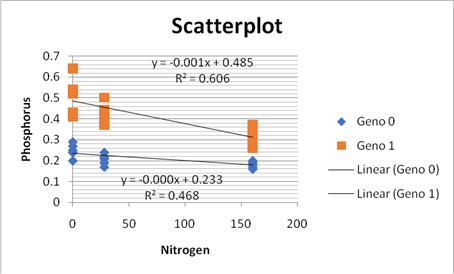
In the scatterplot, we can see that the genotype zero is in red color and genotype one is in blue color. And the lines in the scatterplot are almost parallel so it is linear in nature and in both the lines the points are moving downwards so they are negative in relationship. Thus, as they are parallel so the graph suggest that a multiple regression might be appropriate for these data.
(b)
To use a software to obtain the estimated multiple linear regression equation when the two explanatory variables nitrogen and genotype are included and create a residual plot and explain are the conditions for multiple linear regression satisfied.
(b)
Answer to Problem 28.37E
The estimated multiple linear regression equation is
Explanation of Solution
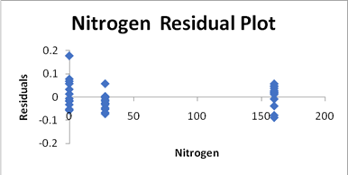
In the question, it is given that an experiment compared the effects of adding various amounts of nitrogen fertilizers to two genotypes of tomato plants, a mild-type and a mutant variety. The percent of phosphorus in the plant, nitrogen and genotype is given in a table. Now, we will use the Excel to obtain the estimated multiple linear regression equation when the two explanatory variables nitrogen and genotype are included and also the residual plot is constructed. We will use the option data analysis in the data tab and run the
| ANOVA | |||||
| df | SS | MS | F | Significance F | |
| Regression | 2 | 0.46916 | 0.23458 | 76.2375 | 4.25E-13 |
| Residual | 33 | 0.10154 | 0.003077 | ||
| Total | 35 | 0.5707 |
| Coefficients | Standard Error | t Stat | P-value | |
| Intercept | 0.256853 | 0.015489 | 16.58326 | 1.43E-17 |
| Nitrogen | -0.00071 | 0.000133 | -5.37461 | 6.11E-06 |
| Genotype | 0.205556 | 0.01849 | 11.11704 | 1.07E-12 |
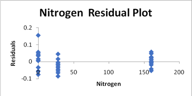
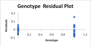
The residual plot will be constructed as:
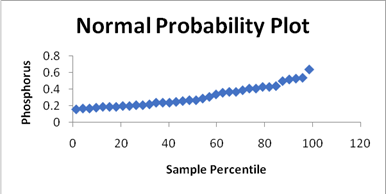
And the normal plot will be constructed as:
Now, the estimated multiple linear regression equation when the two explanatory variables nitrogen and genotype are included is as:
Where
(c)
To create a new variable called interaction by multiplying the explanatory variables nitrogen and genotype and add this new variable to your regression model and provide the estimated multiple linear regression equation and create regression plot for this and discuss whether the conditions for multiple linear regression are met.
(c)
Answer to Problem 28.37E
The conditions for multiple linear regression are met and the estimated multiple linear regression equation is
Explanation of Solution
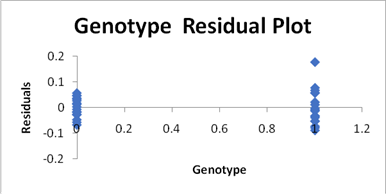
In the question, it is given that an experiment compared the effects of adding various amounts of nitrogen fertilizers to two genotypes of tomato plants, a mild-type and a mutant variety. The percent of phosphorus in the plant, nitrogen and genotype is given in a table. And a new variable called interaction is created by multiplying the explanatory variables nitrogen and genotype. Now, we will use the Excel to obtain the estimated multiple linear regression equation when the two explanatory variables nitrogen and genotype and the interaction are included and also the residual plot is constructed. We will use the option data analysis in the data tab and run the regression analysis. The result will be as:
| ANOVA | |||||
| df | SS | MS | F | Significance F | |
| Regression | 3 | 0.49273 | 0.164243 | 67.4079 | 6.35E-14 |
| Residual | 32 | 0.07797 | 0.002437 | ||
| Total | 35 | 0.5707 |
| Coefficients | Standard Error | t Stat | P-value | |
| Intercept | 0.23387 | 0.015639 | 14.95438 | 5.42E-16 |
| Nitrogen | -0.00035 | 0.000167 | -2.0715 | 0.046455 |
| Genotype | 0.251522 | 0.022117 | 11.37245 | 8.91E-13 |
| Interaction | -0.00073 | 0.000236 | -3.11022 | 0.003912 |
The residual plot is as follows:
The normal plot is as follows:

Now, the estimated multiple linear regression equation when the two explanatory variables nitrogen and genotype and interaction are included is as:
Where
(d)
To explain does the ANOVA table for the model with the interaction term indicate that at least one of the explanatory variables is helpful in predicting the amount of phosphorus in the plant and explain do the individual t tests indicate that all coefficients are significantly different from zero.
(d)
Answer to Problem 28.37E
Yes, the ANOVA table for the model with the interaction term indicates that at least one of the explanatory variables is helpful in predicting the amount of phosphorus in the plant and the individual t tests indicate that all coefficients are significantly different from zero.
Explanation of Solution
In the question, it is given that an experiment compared the effects of adding various amounts of nitrogen fertilizers to two genotypes of tomato plants, a mild-type and a mutant variety. The percent of phosphorus in the plant, nitrogen and genotype is given in a table. Since in the ANOVA table in part (c) we can see that the P-value is less than the level of significance,
Thus, we can say that the ANOVA table for the model with the interaction term indicates that at least one of the explanatory variables is helpful in predicting the amount of phosphorus in the plant. And as we can see in the result of the regression analysis in part (c), we can see that all the P-values are less than the level of significance i.e.
Thus, we have sufficient evidence to conclude that the individual t tests indicate that all coefficients are significantly different from zero.
Want to see more full solutions like this?
Chapter 28 Solutions
Practice of Statistics in the Life Sciences

 MATLAB: An Introduction with ApplicationsStatisticsISBN:9781119256830Author:Amos GilatPublisher:John Wiley & Sons Inc
 Probability and Statistics for Engineering and th...StatisticsISBN:9781305251809Author:Jay L. DevorePublisher:Cengage Learning
 Statistics for The Behavioral Sciences (MindTap C...StatisticsISBN:9781305504912Author:Frederick J Gravetter, Larry B. WallnauPublisher:Cengage Learning
 Elementary Statistics: Picturing the World (7th E...StatisticsISBN:9780134683416Author:Ron Larson, Betsy FarberPublisher:PEARSON
 The Basic Practice of StatisticsStatisticsISBN:9781319042578Author:David S. Moore, William I. Notz, Michael A. FlignerPublisher:W. H. Freeman
 Introduction to the Practice of StatisticsStatisticsISBN:9781319013387Author:David S. Moore, George P. McCabe, Bruce A. CraigPublisher:W. H. Freeman