
Concept explainers
Videos
a.
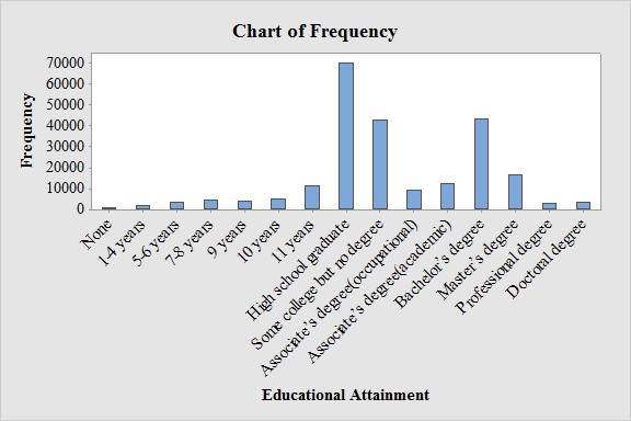
Construct a frequency bar graph.
a.
Answer to Problem 28E
Output obtained from MINITAB software for the educational attainment is:
Explanation of Solution
Calculation:
The given information is a table representing the frequency distribution categorizes U.S. adults aged 18 and over by educational attainment in a year.
Software procedure:
- Step by step procedure to draw the bar chart for educational attainment using MINITAB software.
- Choose Graph > Bar Chart.
- From Bars represent, choose unique values from table.
- Choose Simple.
- Click OK.
- In Graph variables, enter the column of Frequency.
- In Categorical variables, enter the column of Educational Attainment.
- Click OK
Observation:
From the bar graph, it can be seen that the most frequent educational attainment is High school graduate.
b.
Construct a relative frequency distribution for the data.
b.
Answer to Problem 28E
The relative frequency distribution for the data is:
| Educational Attainment | Relative Frequency |
| None | 0.004 |
| 1-4 years | 0.008 |
| 5-6 years | 0.015 |
| 7-8 years | 0.019 |
| 9 years | 0.017 |
| 10 years | 0.020 |
| 11 years | 0.049 |
| High school graduate | 0.300 |
| Some college but no degree | 0.194 |
| Associate’s degree(occupational) | 0.040 |
| Associate’s degree(academic) | 0.052 |
| Bachelor’s degree | 0.184 |
| Master’s degree | 0.071 |
| Professional degree | 0.013 |
| Doctoral degree | 0.014 |
Explanation of Solution
Calculation:
Relative frequency:
The general formula for the relative frequency is,
Therefore,
Similarly, the relative frequencies for the response are obtained below:
| Educational Attainment | Frequency | Relative Frequency |
| None | 834 | |
| 1-4 years | 1,764 | |
| 5-6 years | 3,618 | |
| 7-8 years | 4,575 | |
| 9 years | 4,068 | |
| 10 years | 4,814 | |
| 11 years | 11,429 | |
| High school graduate | 70,441 | |
| Some college but no degree | 42,685 | |
| Associate’s degree(occupational) | 9,380 | |
| Associate’s degree(academic) | 12,100 | |
| Bachelor’s degree | 43,277 | |
| Master’s degree | 16,625 | |
| Professional degree | 3,099 | |
| Doctoral degree | 3,191 |
c.
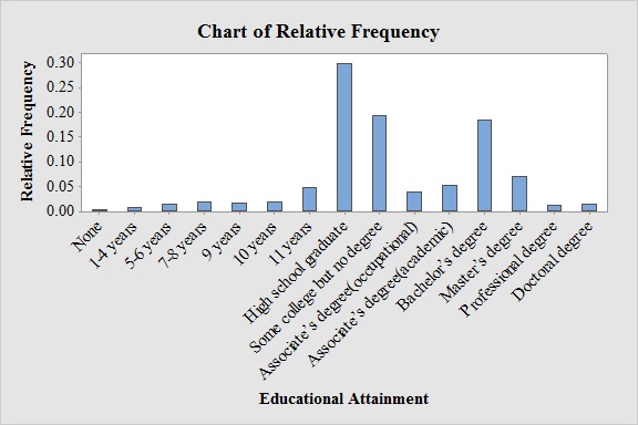
Construct a relative frequency bar graph for these data.
c.
Answer to Problem 28E
Output obtained from MINITAB software for the educational attainment is:
Explanation of Solution
Software procedure:
- Step by step procedure to draw the Bar chart for the response using MINITAB software.
- Choose Graph > Bar Chart.
- From Bars represent, choose unique values from table.
- Choose Simple.
- Click OK.
- In Graph variables, enter the column of Relative Frequency.
- In Categorical variables, enter the column of Educational Attainment.
- Click OK
Observation:
From the graph, it can be seen that most probable educational attainment is High school graduate.
d.
Construct a frequency distribution for the categories 8 years or less, 9-11 years, High school graduate, Some college but no degree, College degree( Associate’s or Bachelor’s), Graduate degree ( Master’s Professional, or Doctoral).
d.
Answer to Problem 28E
The frequency distribution for the data is:
| Educational Attainment | Frequency |
| 8 years or less | 10,791 |
| 9-11 years | 20,311 |
| High school graduate | 70,441 |
| Some college but no degree | 45,685 |
| College degree | 64,757 |
| Graduate degree | 22,915 |
Explanation of Solution
Calculation:
The frequencies for the specified categories are obtained below:
| Educational Attainment | Frequency |
| 8 years or less | |
| 9-11 years | |
| High school graduate | 70,441 |
| Some college but no degree | 42,685 |
| College degree | |
| Graduate degree |
e.
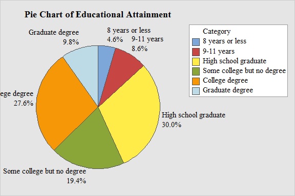
Construct a pie chart for the frequency distribution in part (d).
e.
Answer to Problem 28E
Output obtained from MINITAB software for frequency distribution in part (d) is:
Explanation of Solution
Calculation:
Software procedure:
- Step by step procedure to draw the bar chart for frequency distribution in part (d) using MINITAB software.
- Choose Graph > Pie Chart.
- Choose Chart values from table.
- Under categorical variable, select Educational Attainment.
- Under Summary variables, select Frequency.
- Click OK.
Observation:
There is about 30.0% of the adults are High school graduate and 4.6% of adults are 8 years or less.
f.
Find the proportion of people did not graduate from high school.
f.
Answer to Problem 28E
The proportion of people did not graduate from high school is 0.132.
Explanation of Solution
From the pie chart, it can be seen that there is about 4.6% of the adults are 8 years or less, 8.6% of adults are 9-11 years and all others are graduate from high school. Then the total proportion of people did not graduate from high school is
Hence, the proportion of people did not graduate from high school is 0.132.
Want to see more full solutions like this?
Chapter 2 Solutions
Essential Statistics


 MATLAB: An Introduction with ApplicationsStatisticsISBN:9781119256830Author:Amos GilatPublisher:John Wiley & Sons Inc
 Probability and Statistics for Engineering and th...StatisticsISBN:9781305251809Author:Jay L. DevorePublisher:Cengage Learning
 Statistics for The Behavioral Sciences (MindTap C...StatisticsISBN:9781305504912Author:Frederick J Gravetter, Larry B. WallnauPublisher:Cengage Learning
 Elementary Statistics: Picturing the World (7th E...StatisticsISBN:9780134683416Author:Ron Larson, Betsy FarberPublisher:PEARSON
 The Basic Practice of StatisticsStatisticsISBN:9781319042578Author:David S. Moore, William I. Notz, Michael A. FlignerPublisher:W. H. Freeman
 Introduction to the Practice of StatisticsStatisticsISBN:9781319013387Author:David S. Moore, George P. McCabe, Bruce A. CraigPublisher:W. H. Freeman