
Concept explainers
Videos
Temperatures are measured at various points on a heatedplate (Table P20.60). Estimate the temperature at (a)
TABLE P20.60 Temperatures
|
|
|
|
|
|
|
|
|
100.00 | 90.00 | 80.00 | 70.00 | 60.00 |
|
|
85.00 | 64.49 | 53.50 | 48.15 | 50.00 |
|
|
70.00 | 48.90 | 38.43 | 35.03 | 40.00 |
|
|
55.00 | 38.78 | 30.39 | 27.07 | 30.00 |
|
|
40.00 | 35.00 | 30.00 | 25.00 | 20.00 |
(a)
To calculate: The value of temperature at
| 100.00 | 90.00 | 80.00 | 70.00 | 60.00 | |
| 85.00 | 64.49 | 53.50 | 48.15 | 50.00 | |
| 70.00 | 48.90 | 38.43 | 35.03 | 40.00 | |
| 55.00 | 38.78 | 30.39 | 27.07 | 30.00 | |
| 40.00 | 35.00 | 30.00 | 25.00 | 20.00 |
Answer to Problem 60P
Solution:
The value of temperature at
Explanation of Solution
Given Information:
The data is provided as,
| 100.00 | 90.00 | 80.00 | 70.00 | 60.00 | |
| 85.00 | 64.49 | 53.50 | 48.15 | 50.00 | |
| 70.00 | 48.90 | 38.43 | 35.03 | 40.00 | |
| 55.00 | 38.78 | 30.39 | 27.07 | 30.00 | |
| 40.00 | 35.00 | 30.00 | 25.00 | 20.00 |
Formula used:
The zero-order Newton’s interpolation formula:
The first-order/linear Newton’s interpolation formula:
The second- order/quadratic Newton’s interpolating polynomial is given by,
Where,
The first finite divided difference is,
And, the n th finite divided difference is,
Calculation:
To calculate the temperature
First use the linear interpolation formula and arrange the points as close to about
The values are,
And,
First calculate
Put in above equation,
Similarly for quadratic interpolation,
Now calculate
Put in quadratic interpolation equation,
Now, do it for cubic interpolation by the use of the formula,
Now calculate
Put in cubic interpolation equation,
And, the error is calculated as,
Similarly the other dividend can be calculated as shown above,
Therefore, the difference table can be summarized for
| Order | Error | |
| 0 | 38.43 | 6.028 |
| 1 | 44.458 | |
| 2 | 43.6144 | |
| 3 | 43.368 | |
| 4 | 43.48045 |
Since the minimum error for order third, therefore, it can be concluded that the value of temperature at
(b)
To calculate: The value of temperature at
| 100.00 | 90.00 | 80.00 | 70.00 | 60.00 | |
| 85.00 | 64.49 | 53.50 | 48.15 | 50.00 | |
| 70.00 | 48.90 | 38.43 | 35.03 | 40.00 | |
| 55.00 | 38.78 | 30.39 | 27.07 | 30.00 | |
| 40.00 | 35.00 | 30.00 | 25.00 | 20.00 |
Answer to Problem 60P
Solution:
The value of temperature at
Explanation of Solution
Given Information:
The data is provided as,
| 100.00 | 90.00 | 80.00 | 70.00 | 60.00 | |
| 85.00 | 64.49 | 53.50 | 48.15 | 50.00 | |
| 70.00 | 48.90 | 38.43 | 35.03 | 40.00 | |
| 55.00 | 38.78 | 30.39 | 27.07 | 30.00 | |
| 40.00 | 35.00 | 30.00 | 25.00 | 20.00 |
Formula used:
The zero-order Newton’s interpolation formula:
The first-order/linear Newton’s interpolation formula:
The second- order/quadratic Newton’s interpolating polynomial is given by,
Where,
The first finite divided difference is,
And, the n th finite divided difference is,
Calculation:
To calculate the temperature
Since, this is a two-dimensional interpolation, therefore one way is to use cubic interpolation along the y direction for specific values of x and then go along the x direction for values of y obtained from the previous analysis.
First use the linear interpolation formula and arrange the points as close to about
The values are,
And,
First calculate
Put in above equation,
Similarly for quadratic interpolation,
Now calculate
Put in quadratic interpolation equation,
Now, do it for cubic interpolation by the use of the formula,
Now calculate
Put in cubic interpolation equation,
And, the error is calculated as,
Similarly the other dividend can be calculated as shown above,
Therefore, the difference table can be summarized for
| Order | Error | |
| 0 | 64.49 | |
| 1 | 59.0335 | |
| 2 | 58.411 | |
| 3 | 58.47032 |
Now, do this for
The values are,
And,
First calculate
Put in above equation,
Similarly for quadratic interpolation,
Now calculate
Put in quadratic interpolation equation,
Now, do it for cubic interpolation by the use of the formula,
Now calculate
Put in cubic interpolation equation,
Similarly, for
Now for the calculation for
The values are,
And,
First calculate
Put in above equation,
Similarly for quadratic interpolation,
Now calculate
Put in quadratic interpolation equation,
Now, do it for cubic interpolation by the use of the formula,
Now calculate
Put in cubic interpolation equation,
And, the error is calculated as,
Similarly the other dividend can be calculated as shown above,
Therefore, the difference table can be summarized for
| Order | Error | |
| 0 | 47.15 | |
| 1 | 46.4885 | |
| 2 | 46.0479875 | |
| 3 | 46.140425 |
Hence, the value of temperature at
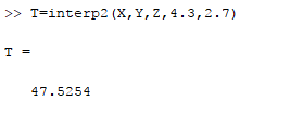
This problem can also be solved with MATLAB as it contains the predefined function interp2.
The MATLAB code is as shown below,
The output in the command window is,
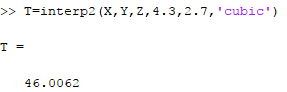
For more accuracy, the result can also be obtained from the bicubic interpolation as shown below,
Finally, the interpolation can also be implemented with the use of splines as shown below,
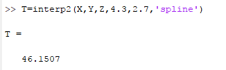
Hence, it can be concluded that the result is similar to that obtained from the calculation.
Want to see more full solutions like this?
Chapter 20 Solutions
EBK NUMERICAL METHODS FOR ENGINEERS


- Project 1 100 20. 150 200 250 300 350 400 450 500 550 600 650 QUPINHFC-134a 700 200. 00012 00013 0.0014 r0.0016 J00018 10. Pressure-Enthalpy 0.0020 8. 0.0030 100. 80. 6. Diagram volume 0.0040 mikg (SI Units) 0.0060 0 0080 0.010 4. 60. 40. 2. 0.015 0 020 20. 1. 0.8 0030 0.040 10. 8. 0.6 0.060 0.4 6. 0.080 010 0.2 0.15 020 2. 0.1 0.30 0.08 0.40 1. 0.8 0.06 060 0.04 0.6 O80 1.0 0.4 0.02 15 20 0.2 0.01 100 150 200 250 300 350 400 450 0.1 700 500 550 600 650 Enthalpy (kJ/kg) Refrigerant HFC-134a as the working fluid Ideal cycle operation condition is assumed - Cycle is operated at high pressure line of 0.8 MPa - Cycle is operated at low temperature line of – 10° C - Flow rate is 0.1 kg/sec The head of the department in the company that you are working in asked you to make use of pressure -enthalpy chart provided for HFC-134a refrigerant Task.1 1. Determine the Refrigeration effect (RE), heat of compression (HOC), and heat of rejection (HOR) and their corresponding rate/power values in kW.…arrow_forward3. Examine your data in Data Table 2 and in Data Table 3. For the data with the smallest percentage difference, compare the total energy at each point. Calculate the sum U₁+Ug at x₁ as ½kx-mgx₁. Calculate that sum at x₂ as ½kx²-mgx₂. Do you expect them to agree reasonably well? Explain why they should or should not be the same. 4. Consider the same data as used in Question 3. Calculate the value of x halfway between x₁ and x₂. Calculate U₁+Ug=½kx² − mgx_for_that point. Do you expect them to agree with the energy calculated in Question 3? If they agree reasonably well, explain why they do. If they do not agree, explain why they do not agree.arrow_forward100 80 60 40 20 0.002 0.004 0.006 0.008 0.01 0.012 Strain, in/in. FIGURE P1.17 1.18 Use Problem 1.17 to graphically determine the following: a. Modulus of resilience b. Toughness Hint: The toughness (u) can be determined by calculating the area under the stress-strain curve u = de where & is the strain at fracture. The preceding integral can be approxi- mated numerically by using a trapezoidal integration technique: u, = Eu, = o, + o e, - 6) %3D c. If the specimen is loaded to 40 ksi only and the lateral strain was found to be -0.00057 in./in., what is Poisson's ratio of this metal? d. If the specimen is loaded to 70 ksi only and then unloaded, what is the permanent strain? Stress, ksiarrow_forward
- In the Fig. 2 below, let Ki = K2 = K and ti = t=t. %3D T -T X Fig. 2 (a) Let T= 0 °C and T= 200 °C. Solve for T: and unknown rates of heat flow in term of k and t. MEC_AMO_TEM_035_02 Page 2 of 11 Finite Element Analysis (MECH 0016.1) – Spring - 2021 -Assignment 2-QP (b) Let T- 400 °C and let fs have the prescribed value f. What are the unknowns? Solve for them in term of K, t, and f.arrow_forward(SI units) Aluminum has a density of 2.70g/cm³ at room temperature (20°C). Determine its density at 650°C, using data in Table 4.1 for reference.arrow_forwardSample Paychrometrie Chart (Use the Chart from the Weather ToolKit 6.0 WET BULB (WB) TEMPERATURE 5.5 35 5.0 作30 4.5 300 4.0 25 HMIDI 3.5 20 3.0 2.5 15 20 68% 2.0 S0% 1.5 10 (kPa) 100 1.0 20% 0.5 10% 0.0 -10-5 0 5 10 15 20 25 30 35 40 DRY BULB TEMPERATURE (Celsius) At a temperature of 25 °C what is the mixing ratio if the relative humidity is E Work from the printed chart from the Tools folder O a) 12.5 g/kg Ob) 16.5 g/kg O) 18.5 g/kg O d) 20 g/kg O e) 22.5 g/kg VAPOUR UREarrow_forward
- The following related values of the pressure p in kN/m2 and the volume V in cubic meter where measured from the compression curve of an internal combustion engine indicator diagram. Assuming that P and V are connected by the law PVn: C, find the value of n. p 3450 2350 1725 680 270 130 V .0085 .0113 .0142 .0283 .0566 .0991arrow_forwardQI) The vapour pressure, p, of nitric acid varies with temperature as follows: 0 20 40 1.92 6.38 17.7 27.7 62.3 89.3 124.9 170.9 50 70 80 90 100 p/kPa What are : (a) the normal boiling point (b) the enthalpy of vaporization of nitric acid? Q2) Calculate the melting point of ice under a pressure of 50 bar. Assume that the density of ice under these conditions is approximately 0.92 g cm and that of liquid water is 1.00 g em'. Q3) An open vessel containing (a) water, (b) benzene, (e) mercury stands in a laboratory measuring 5.0 m x 5.0 m x 3.0 m at 25°C. What mass of each substance will be found in the air if there is no ventilation? (The vapour pressures are (a) 3.2 kPa, (b) 13.1 kPa, (c) 0.23 Pa.)arrow_forwardFor an ideal gas if the specific internal energy at a specific pressure and temperature of 20 °C is u=235.9 kJ/kg, what is the specific internal energy if the pressure is doubled while the temperature stays the same. Select one: a. 117.95 b. 235.90 c. 353.85 d. 707.70 e. 471.80arrow_forward
- Stress, a (MPa) Strain, e (x10* m/m) Yong Modulus, E (GPa) 3.963 40.0 99.1 7.926 75.0 106 11.89 105.0 113.2 1.85 122.0 130.0 19.81 144,0 137.6 Table 2 Stress and Strain 3|Page Dissections 1. Draw the graph of stress against strain 2. Discusses the obtained results 3. From the graph find. stress ? Yong Modulus, E? 4. Why Compression test is important in industry ?arrow_forwardA silver cube with an edge length of 2.24 cm and a gold Substance Specific heat (J/g.°C) Density (g/cm³) cube with an edge length of 2.63 cm are both heated to gold 0.1256 19.3 84.8 °C and placed in 115.0 mL of water at 20.5 °C . silver 0.2386 10.5 What is the final temperature of the water when thermal water 4.184 1.00 equilibrium is reached? Tinalarrow_forwardSaturated steam at 99.6 °C is heated to 350°C. Use the steam table provided to determine: a. The required heat input if 1 kg of steam undergoes the process in a variable-volume constant-pressure container. b. The work of expansion (in kJ) of the steam undergoing the process. C. The required heat input if a continuous stream flowing at 1 kg/s undergoes the process at constant pressure. d. Does your numeric answer to part c equal the sum of parts b and a? Explain why or why not. Given: 1 bar = 10 N/m4, Q= AH, Q = AU, AA = AÛ + PAV, table B.7 in kJ/kg and m/kg.arrow_forward
 Elements Of ElectromagneticsMechanical EngineeringISBN:9780190698614Author:Sadiku, Matthew N. O.Publisher:Oxford University Press
 Mechanics of Materials (10th Edition)Mechanical EngineeringISBN:9780134319650Author:Russell C. HibbelerPublisher:PEARSON
 Thermodynamics: An Engineering ApproachMechanical EngineeringISBN:9781259822674Author:Yunus A. Cengel Dr., Michael A. BolesPublisher:McGraw-Hill Education
 Control Systems EngineeringMechanical EngineeringISBN:9781118170519Author:Norman S. NisePublisher:WILEY
 Mechanics of Materials (MindTap Course List)Mechanical EngineeringISBN:9781337093347Author:Barry J. Goodno, James M. GerePublisher:Cengage Learning
 Engineering Mechanics: StaticsMechanical EngineeringISBN:9781118807330Author:James L. Meriam, L. G. Kraige, J. N. BoltonPublisher:WILEY