
Concept explainers
Videos
Soft tissue follows an exponential deformation behavior in uniaxial tension while it is in the physiologic or normal range of elongation. This can be expressed as
where
To evaluate
In the following table is stress-strain data for heart chordate tendineae (small tendons used to hold heart valves closed during contraction of the heart muscle; these data are from loading the tissue, while different curves are produced on unloading).
|
|
87.8 | 96.6 | 176 | 263 | 351 | 571 | 834 | 1229 | 1624 | 2107 | 2678 | 3380 | 4258 |
|
|
153 | 204 | 255 | 306 | 357 | 408 | 459 | 510 | 561 | 612 | 663 | 714 | 765 |
Calculate the derivative
Plot the stress versus strain data points along with the analytic curve expressed by the first equation. This will indicate how well the analytic curve matches these data.
Many times this does not work well because the value of
Using this approach, experimental data that are well defined will produce a good match of the data points and the analytic curve. Use this new relationship and again plot the stress versus strain data points and this new analytic curve.
To calculate: The values of
Answer to Problem 16P
Solution: The function that fits the data perfectly is
Explanation of Solution
Given Information:
The provided values of the stress
| 87.8 | 96.6 | 176 | 263 | 351 | 571 | |
| 153 | 204 | 255 | 306 | 357 | 408 |
And,
| 834 | 1229 | 1624 | 2107 | 2678 | 3380 | 4258 | |
| 459 | 510 | 561 | 612 | 663 | 714 | 765 |
Formula Used:
The formula for the derivative of a function at a point c using forward difference is:
The formula for the derivative of a function at a point c using backward difference is:
The formula for the derivative of a function at a point c using central difference is:
Calculation:
Consider the formula for the stress:
Differentiate both sides with respect to
This is a linear equation.
First obtain the value of the derivative of the stress
Now the derivative at the second data point can be obtained using the central difference. Note that the data is equally spaced with a step-size of 51.
Now do the same for all the data points except the last one:
And,
And,
And,
And,
Now the derivative at the last data point can be obtained using the backward difference. Note that the data is equally spaced with a step-size of 51.
Hence, the derivatives have been obtained as:
Now perform a regression analysis on the derivative with respect to
This can be done using MS-Excel.
Step 1: Enter the data points in a blank workbook.
Step 2: Select the data points, go to insert and the select scatter plot.
This gives:
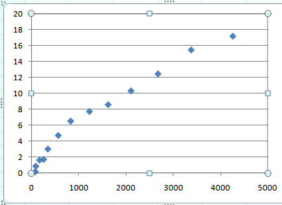
It can be seen that the first four points do not follow a linear relationship. So disregard the first four points and obtain a line of best fit for the remaining points.
This can be done using MATLAB.
Code:
Output:
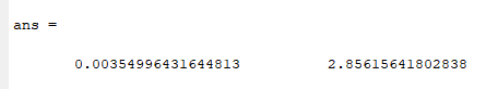
This implies that the linear model for the derivative is:
This gives the value of a as 0.0035499643 and the value of
Now, substitute this in the formula for stress to obtain:
To check whether this model is a good fit for the data, plot this model along with the provided data points. This can be done using MATLAB.
Code:
Output:
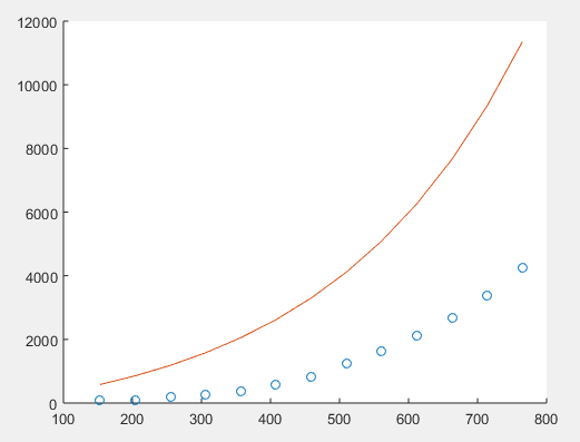
Clearly, the obtained function is not a good fit for the data.
Rewrite the expression for the original functionto obtain:
Use this to obtain:
Now consider a data point in the middle of the data
Use this to get the formula for the strain as:
To check whether this model is a good fit for the data, plot this model along with the provided data points. This can be done using MATLAB.
Code:
Output:
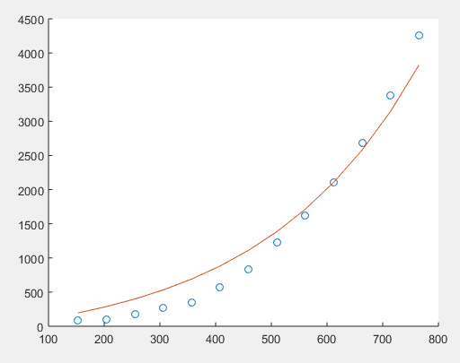
It is clear that the function obtained using the data point from the middle is a much better fit for the provided data points.
Hence, the desired function that fits the data points is
Want to see more full solutions like this?
Chapter 20 Solutions
EBK NUMERICAL METHODS FOR ENGINEERS
Additional Engineering Textbook Solutions
Basic Technical Mathematics
Fundamentals of Differential Equations (9th Edition)
Advanced Engineering Mathematics
College Algebra (6th Edition)
Statistics Through Applications


- The following data were recorded during the tensile test of a test specimen with a diameter of 12.8 mm. The gage length is 50.8 mm. The given data are as follow; Given: Test specimen material: Aluminum Diameter of test specimen: Do = 12.8 mm Length of test specimen: Lo = 50.8 mm Force and Elongation data for test specimen Assumptions: 1. The given data is accurate and the material is isotropic 2. The direction of applied force is parallel to the length of the cylinder Requirement: To interpret and plot the stress Vs Strain curve for a given specimen DATA: LENGTH, mm STRESS, MPa LOAD, N 0 50.8 7 330 50.851 15 100 50.902 23 100 50.952 30 400 51.003 34 400 51.054 38 400 51.308 41 300 51.816 44 800 52.832 46 200 53.848 47 300 54.864 47 500 55.88 36 100 56.896 44 800 57.658 42 600 58.42 36 400 59.182 STRAINarrow_forward6. State your answers to the following questions.Strain Gauge represents the deformation of a material through a change in resistance. If so, explain how temperature will affect the strain gauge in the experimental environment.①:In this experiment, the Strain Gauge measures the strain in micro units. Explain one possible error factor when applying a load by hanging a weight on the material with the strain gauge attached. (Hint: It is easy to shake by hanging the weight using a thread)①:arrow_forward1. A tension test on an aluminum plate resulted in the following engineering stress-engineering strain data as reported in the first and second column of the table below (reduction of area, RA=17%): S (psi) e (in/in) σ (psi) ε (in/in) 10500 0.001 10510.5 0.000995 21000 0.002 31200 0.003 41300 0.004 51200 0.005 61200 0.006 70600 0.007 74700 0.0075 76800 0.008 77600 0.0085 78000 0.009 78400 0.0095 78700 0.01 81200 0.02 83000 0.03 84200 0.04 85400 0.05 86200 0.06 86800 0.07 *87200 0.08 **86200 0.1 Note: * maximum load, ** load at fracture a) Calculate the corresponding true stress and true strain and give your results in a table along with the engineering stress, engineering strain shown in the of table above (column 3 and 4). b) Plot the true stress-true strain curve on a rectangular coordinate. c) Plot the true stress-true strain curve on a log-log graph and determine the plastic flow curve parameters K and n, the yield strength, Y, and the elastic modulus, E of the material.arrow_forward
- 650 600 550 500 450 400 350 300 250 200 150 100 50 0.002 0.004 0.006 0.008 0.01 0.012 0.014 0.016 0.018 0.02 Strain mm/mm The graph above shows the stress-strain relationship of a steel bar under tension test. The steel bar diameter = 8 mm and the bar gauge length = 100 mm. Determine the following: If the specimen is loaded to 550 MPa and then unloaded. What would be the modulus of resilience of the sample after reloading? Stress (MPa)arrow_forwardThe stress-strain curve for a material is shown below. The modulus of toughness for this material is most closely equal to: σ (ksi) 105 90 75 60 8 45 30 15 0 0 0.05 0.10 0.15 0.20 0.25 0.30 0.35 0 0.001 0.002 0.003 0.004 0.005 0.006 0.007 28 ksi 16 ksi 38 ksi 22 ksi € (in./in.)arrow_forwardYoung Modulus of a material has characteristics of : (Choose TRUE or FALSE for each statement) Can be obtained by the gradient of stress versus strain graph. OTRUE OFALSE As a measurement for a material due to its resistance, subjected to the exerted forces. O TRUE O FALSE The two-dimensional plane of the material depends on Young Modulus. O TRUE OFALSEarrow_forward
- QUESTION 2' a) When a strain gauge is stretched under axial tension, its resistance varies with the imposed strain. A resistance bridge circuit is used to convert the resistance change into voltage as shown in Figure 2. i) Distinguish among stress and strain. ii) In Figure 2, the 120 22 strain gauge with a gauge factor of 2 is mounted on a rectangular steel bar (Em = 200 GPa, 3 cm wide and 1 cm high) and connected to bridge circuit with input voltage, E₁=5 V. If the voltmeter shows 1.25 mV, calculate the amount of tensile load applied to the steel bar. Gauge axis Figure 2 E Tensile loading 3cm 1 cmarrow_forwardThe following data are taken from a 20mm in diameter bar of length 250mm, the following results were recorded. Assume that the curve of the stress-strain diagram is linear from the origin to the first point. P (load in kN) 8(elongation in mm) 112 0.2 154 0.3 167 0.4 0.5 174 181 0.8 Determine the a. Stress at 187 kN load in MPa b. Strain at 167 kN load in mm/mm (expressed in scientific notation) c. Modulus of elasticity in MPa d. Modulus of resilience in N-mm/mm e. Modulus of toughness in N-mm/mm 234 oo OOO O0arrow_forwardAnswer must be coorect -- when using three-wire connections to a strain gage to reduce the effects of leadwire resistance changes with temperature, a phenomenon called leadwire desensitization can occur. If the magnitude of the leadwire resistance exceeds 0.1% of the nominal gage resistance, significant error can result. Assuming a 18-gauge (AWG) platinum leadwire (resistivity 10.6×10⁻⁸ S2m) and a standard 120 22 gage, how long can the (individual) leads (in inches) be before there is leadwire desensitization?arrow_forward
- Data taken from a stress-strain test for a ceramic are given in the table. The curve is linear between the origin and the first point. Figure σ (ksi) 0 33.2 45.5 49.4 51.5 53.4 € (in./in.) 0 0.0006 0.0010 0.0014 0.0018 0.0022 < 1 of 1 Part A Plot the stress-strain diagram. (Figure 1) +SGA0 No elements selected σ(ksi) Submit Request Answer 50 40 30+ 20 10 0.5 1.0 1.5 2.0 2.5 €x 10-³(in./in.) ? Select the elements from the list and add them to the canvas setting the appropriate attributes. Press [CTRL+M) to get to the main menu.arrow_forwardA 1045 hot-rolled steel tension test specimen has the original diameter and length of 6 mm and 25 mm, respectively. The load and change in length data were recorded as shown in Table 1 below: Table 1. Load and change in length Load (KN) Change in Length Load (KN) Change in Length (mm) |(mm) 20.56 2.26 2.94 0.01 20.72 3.36 5.58 0.02 20.61 3.83 8.52 0.03 19.97 4.00 11.16 0.04 18.72 Fracture. 12.63 0.05 13.02 0.06 13.16 0.08 13.22 0.10 16.15 0.61 18.50 1.04 20.27 1.80arrow_forward1. A cylindrical specimen of a metal object with a radius of 3.8E-2 m and a gauge length of 20.31 mm is pulled in tension. Use the load-elongation characteristics tabulated below to answer the following questions; Load Length (N) (mm) 20.31 20.38 12 20.45 18 20.51 24 20.55 30 20.61 36 20.64 42.8 20.68 48.9 20.72 55.2 20.76 60 20.79 65.8 20.84 70.7 20.87 77.3 20.93 83.1 20.98 88.6 22.15 91.58 23.24 91.68 25.41 0 6 Change in length Length (x10-2 m) (m) Computed strain Computed stress (N/m²) (a) Compute the cross-sectional area of brass. (3arrow_forward
 Elements Of ElectromagneticsMechanical EngineeringISBN:9780190698614Author:Sadiku, Matthew N. O.Publisher:Oxford University Press
 Mechanics of Materials (10th Edition)Mechanical EngineeringISBN:9780134319650Author:Russell C. HibbelerPublisher:PEARSON
 Thermodynamics: An Engineering ApproachMechanical EngineeringISBN:9781259822674Author:Yunus A. Cengel Dr., Michael A. BolesPublisher:McGraw-Hill Education
 Control Systems EngineeringMechanical EngineeringISBN:9781118170519Author:Norman S. NisePublisher:WILEY
 Mechanics of Materials (MindTap Course List)Mechanical EngineeringISBN:9781337093347Author:Barry J. Goodno, James M. GerePublisher:Cengage Learning
 Engineering Mechanics: StaticsMechanical EngineeringISBN:9781118807330Author:James L. Meriam, L. G. Kraige, J. N. BoltonPublisher:WILEY