
Videos
Human blood behaves as a Newtonian fluid (see Prob. 20.55) in the high shear rate region where
where
|
|
0.91 | 3.3 | 4.1 | 6.3 | 9.6 | 23 | 36 | 49 | 65 | 105 | 126 | 215 | 315 | 402 |
|
|
0.059 | 0.15 | 0.19 | 0.27 | 0.39 | 0.87 | 1.33 | 1.65 | 2.11 | 3.44 | 4.12 | 7.02 | 10.21 | 13.01 |
| Region | Casson | Transition | Newtonian |
Find the values of
To calculate: The values of
| 0.91 | 3.3 | 4.1 | 6.3 | 9.6 | 23 | 36 | 49 | 65 | 105 | 126 | 215 | 315 | 402 | |
| 0.0059 | 0.15 | 0.19 | 0.27 | 0.39 | 0.84 | 1.33 | 1.65 | 2.11 | 3.44 | 4.12 | 7.02 | 10.21 | 13.01 | |
| Region | Casson | Transition | Newtonian | |||||||||||
Also, find the correlation coefficient for each regression analysis. Plot the two regression lines on the Casson plot (
) and extend the regressions lines as dashed lines into adjoining regressions and include the given data points in the plots.
Answer to Problem 15P
Solution: In the Casson region
and in Newtonian region
and in Newtonian region
Explanation of Solution
Given Information: Consider the experimentally measured values of
| 0.91 | 3.3 | 4.1 | 6.3 | 9.6 | 23 | 36 | 49 | 65 | 105 | 126 | 215 | 315 | 402 | |
| 0.0059 | 0.15 | 0.19 | 0.27 | 0.39 | 0.84 | 1.33 | 1.65 | 2.11 | 3.44 | 4.12 | 7.02 | 10.21 | 13.01 | |
| Region | Casson | Transition | Newtonian | |||||||||||
The Casson relationship is with
The relationship for the Newtonian fluid,
Formula used:
If
data points
Here,
If
data points
The correlation coefficient is,
Here,
Calculation:
Consider the experimentally measured values of
| 0.91 | 3.3 | 4.1 | 6.3 | 9.6 | 23 | 36 | 49 | 65 | 105 | 126 | 215 | 315 | 402 | |
| 0.0059 | 0.15 | 0.19 | 0.27 | 0.39 | 0.84 | 1.33 | 1.65 | 2.11 | 3.44 | 4.12 | 7.02 | 10.21 | 13.01 | |
| Region | Casson | Transition | Newtonian | |||||||||||
The Casson relationship is with
Defining the two variables
Therefore, the unknown constant
Construct the following table considering the data in the Casson regions to compute the unknown constant
| 1 | 0.91 | 0.0059 | 0.95394 | 0.07681 | 0.91000 | 0.07327 |
| 2 | 3.3 | 0.15 | 1.81659 | 0.38730 | 3.30000 | 0.70356 |
| 3 | 4.1 | 0.19 | 2.02485 | 0.43589 | 4.10000 | 0.88261 |
| 4 | 6.3 | 0.27 | 2.50998 | 0.51962 | 6.30000 | 1.30422 |
| 5 | 9.6 | 0.39 | 3.09839 | 0.62450 | 9.60000 | 1.93494 |
| 6 | 23 | 0.84 | 4.79583 | 0.91652 | 23.00000 | 4.39545 |
| 7 | 36 | 1.33 | 6.00000 | 1.15326 | 36.00000 | 6.91954 |
| 21.19957 | 4.11389 | 83.21000 | 16.21360 |
Therefore, the unknown constant
Therefore,
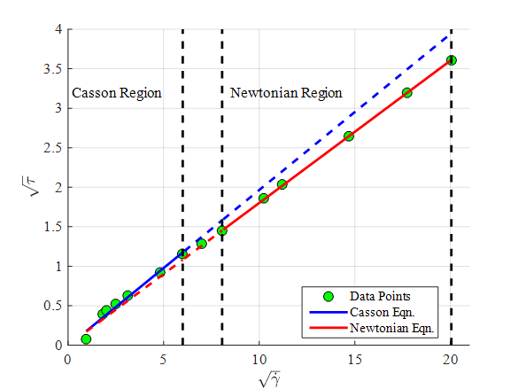
Hence, the linear regression line for Casson region is,
Construct the table to calculate the correlation coefficients defining
| 1 | 0.95394 | 0.07681 | 0.26101 | 0.17789 | 0.01022 |
| 2 | 1.81659 | 0.38730 | 0.04016 | 0.34830 | 0.00152 |
| 3 | 2.02485 | 0.43589 | 0.02305 | 0.38944 | 0.00216 |
| 4 | 2.50998 | 0.51962 | 0.00463 | 0.48527 | 0.00118 |
| 5 | 3.09839 | 0.62450 | 0.00135 | 0.60151 | 0.00053 |
| 6 | 4.79583 | 0.91652 | 0.10812 | 0.93682 | 0.00041 |
| 7 | 6.00000 | 1.15326 | 0.31986 | 1.17469 | 0.00046 |
| 0.75818 | 0.01648 |
Therefore,
Hence, the correlation coefficients,
Therefore, for Casson region the linear fit is,
And the correlation coefficients,
Consider the Newtonian relationship as,
From the linear regression,
Construct the following table considering the data in the Newton regions to compute the unknown constant
| 1 | 105 | 3.44 | 11025 | 361.20 |
| 2 | 126 | 4.12 | 15876 | 519.12 |
| 3 | 215 | 7.02 | 46225 | 1509.30 |
| 4 | 315 | 10.21 | 99225 | 3216.15 |
| 5 | 402 | 13.01 | 161604 | 5230.02 |
| 37.8 | 333955 | 10835.79 |
Therefore, the unknown constant
Therefore,
Hence, the linear regression line for Newtonian region is,
Construct the table to calculate the correlation coefficients defining
| 1 | 105 | 3.44 | 16.97440 | 3.40725 | 0.00107 |
| 2 | 126 | 4.12 | 16.97440 | 4.08870 | 0.00098 |
| 3 | 215 | 7.02 | 49.28040 | 6.97675 | 0.00187 |
| 4 | 315 | 10.21 | 104.24410 | 10.22175 | 0.00014 |
| 5 | 402 | 13.01 | 169.26010 | 13.04490 | 0.00122 |
| 356.73340 | 0.00528 |
Therefore,
Hence, the correlation coefficients,
Therefore, for Newtonian region the linear fit is
And the correlation coefficients,
Graph:
Consider the two regression lines in the field of
In the Casson region,
In the Newtonian region,
Construct the MATLAB function ‘Code_97924_20_15a.m’ to plot the two regression lines on the Casson plot (
) and extend the regressions lines as dashed lines into adjoining regressions and include the given data points in the plots.
The comparison is shown on the plot as,
Want to see more full solutions like this?
Chapter 20 Solutions
EBK NUMERICAL METHODS FOR ENGINEERS


- Two-dimensional irrotational fluid flow is conveniently described by a complex poten- tial f(z) = u(x, v) + iv(x, y). We label the real part, u(x, y), the velocity potential, and the imaginary part, v(x, y), the stream function. The fluid velocity V is given by V = Vu. If f(z) is analytic: 11.2.11 (a) Show that df/dz= Vx – i Vy. (b) Show that V · V = 0 (no sources or sinks). (c) Show that V x V=0 (irrotational, nonturbulent flow).arrow_forwardIn a fluid flow, the density of the fluid is constant for incompressible flow Select one: True Falsearrow_forward4. For steady laminar flow, the reduction in (d(p + yh)/dx ) represents the work done on fluid per unit volume. The work done is converted into irreversibilities (losses) by the action of viscous shear. Thus, the net work done and the loss of potential energy represents the losses per unit time due to irreversibilities. How can we calculate this net power?arrow_forward
- For the flow of a viscous fluid, with the velocity V = f(x)g(y)h(z)i (where f, g, h are arbitrary functions), the following conditions are given: . The flow is adiabatic. • The quantities v = 2 and 3 = $ are constants. • The velocity circulation is conserved for the flow, irrespective of the values of vand 3. What is the general solution for the functions f, g, h?arrow_forward1. Answer the following questions: (a) What is the physical meaning of the following: D a +V.v at Dt where V is the velocity vector of the flow field. (b) Let the viscous stress tensor be denoted by 7. How is the surface (vector) force f, acting by the fluid on a surface element ds (with unit normal în ) computed? Give your answer in vector notation and also in index notation. What is the physical meaning of Ty ? (c) Write down the work done on a material volume of fluid by the viscous surface force in vector notation and also in index notation. (d) Write down the amount of conduction heat flux 'q' (a scalar) on a surface element ds (with unit normal în ) in vector notation and also in index notation.arrow_forwardThe flow between two horizontal infinite parallel plates is a two-dimension, steady-state, incompressible and fully- developed flow. The distance between the plates is h m. The bottom plate is stationary and the top plate velocity is U. m/s in the x-direction. The flow is driven by the top moving plate and there is, therefore, no pressure gradient in the direction of the flow. Velocity in the y-direction, v = 0. Note: Align the x-axis to the bottom wall. Use the x-momentum equation to show that the velocity profile equation is (a) u(y) = ay + b and find the values of a and b. Use the energy equation to derive the temperature distribution T(y) for the flow if the surface temperature and temperature gradient on the bottom plate are both zero. (b)arrow_forward
- Q.5 A plate 1 mm distance from a fixed plate, is moving at 500 mm/s by a force induces a 2 shear stress of 0.3 kg(f)/m. The kinematic viscosity of the fluid (mass density 1000 kg/ 3. m) flowing between two plates (in Stokes) isarrow_forwardQ: Consider the unsteady mass conservation equation (1.5) as it might describe the flow accelerating through a duct with a variable cross section. If the largest velocity gradient measured locally is du/dx and the largest density gradient is dpldx, what order-of-magnitude relationship must exist between du/dx and dpldx for the simplified equation (1.8) to be applicable? ap ap +p ax ap ap du av Hint 1: aw + = 0 az +u at ax (1.5) + v. +w. ду az ду du aw Hint 2: ax (1.8) дуarrow_forwardQ2 The airflow in large wind tunnels is driven by large fans that exert a thrust force on their support structure. The thrust force, F, on a support structure can be expected to be a function of the density and viscosity of the air, the size of the fan, and the rate at which the fan rotates. Determine a nondimensional functional expression that relates the thrust generated by a fan to the influencing variables. F = f(D, Q, w, p, μ)arrow_forward
- The velocity along the centreline of a nozzle of length L is given by 2L v = velocity in m/s; t = time in seconds; x = distance from inlet of nozzle where, %3D The total acceleration in m/s?, when t = 3s, x = 0.5 m and L = 1 m, is %3Darrow_forwardQ2 The airflow in large wind tunnels is driven by large fans that exert a thrust force on their support structure. The thrust force, F, on a support structure can be expected to be a function of the density and viscosity of the air, the size of the fan, and the rate at which the fan rotates. Determine a nondimensional functional expression that relates the thrust generated by a fan to the influencing variables. F = f(D, Q, w, p, μ) Quantity Dimension Q L³T-1 V LT-1 D,H,W,I L Р ML-3 μ ML-¹T-1 ML-¹T-2 MLT-² T-1 ML²T-² L²T-² P F (0) E e(=E/m)arrow_forwardIn the field of air pollution control, one often needs to sample the quality of a moving airstream. In such measurements a sampling probe is aligned with the flow as sketched in Fig. A suction pump draws air through the probe at volume flow rate V· as sketched. For accurate sampling, the air speed through the probe should be the same as that of the airstream (isokinetic sampling). However, if the applied suction is too large, as sketched in Fig, the air speed through the probe is greater than that of the airstream (super iso kinetic sampling). For simplicity consider a two-dimensional case in which the sampling probe height is h = 4.58 mm and its width is W = 39.5 mm. The values of the stream function corresponding to the lower and upper dividing streamlines are ?l = 0.093 m2/s and ?u = 0.150 m2/s, respectively. Calculate the volume flow rate through the probe (in units of m3/s) and the average speed of the air sucked through the probe.arrow_forward
 Principles of Heat Transfer (Activate Learning wi...Mechanical EngineeringISBN:9781305387102Author:Kreith, Frank; Manglik, Raj M.Publisher:Cengage Learning