
Concept explainers
Videos
a.
Find the expected value of change in biomass concentration associated with a 1-day increase in elapsed time.
a.
Answer to Problem 53CR
A one day increase in elapsed time will decrease the biomass concentration by
Explanation of Solution
Calculation:
It is given that y is the green biomass concentration
The simple linear equation is given as follows:
The above regression equation can be interpreted as, 1 unit increase of x will lead to decrease of 0.64 units in y, due to the negative slope of x.
Thus, 1 day increase in elapsed time will decrease the biomass concentration by
b.
Find the predicted value of biomass concentration if elapsed time is 40 days.
b.
Answer to Problem 53CR
The predicted value of biomass concentration for an elapsed time of 40 days is
Explanation of Solution
Calculation:
From Part (a), the regression equation is given by:
Substitute
Thus, the predicted value of biomass concentration for elapsed time of 40 days is
c.
Check whether there is a linear relationship between the two variables or not.
c.
Answer to Problem 53CR
There is convincing evidence of a useful linear relation between elapsed time and biomass concentration.
Explanation of Solution
Calculation:
It is given that the coefficient of determination
Denote
The null and alternative hypotheses are given by:
That is, there is no linear relationship between x and y.
That is, there is a linear relationship between x and y.
Assume that the level of significance for the test is
The test statistic for t–test when coefficient of determination is known is given by:
The quantity,
Here, the r value can be considered as negative, because the regression coefficient has negative value. Thus, the acceptable value of r is,
By substituting the values in the test statistic formula, one can get the value of test statistic.
That is,
Software procedure:
Step-by-step procedure to find the P-value using the MINITAB software:
- Choose Graph > Probability Distribution Plot.
- Choose View Probability > OK.
- From Distribution, choose ‘t’ distribution.
- Enter the Degrees of freedom as 56.
- Click the Shaded Area tab.
- Choose X Value and Both Tails for the region of the curve to shade.
- Enter the X value as –7.047.
- Click OK.
Output obtained using the MINITAB software is represented as follows:
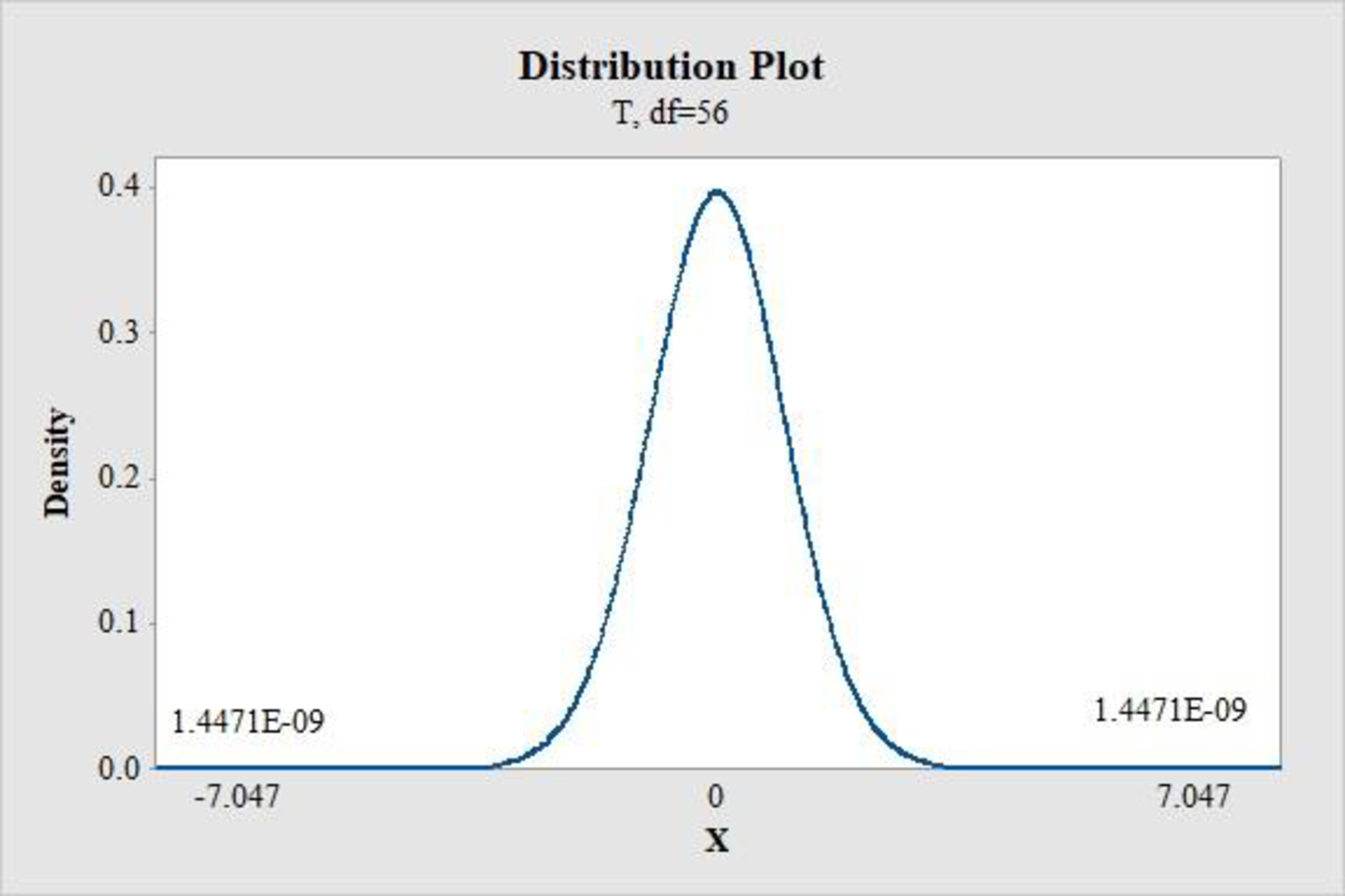
From the above graph, P-value is given by 1.4471E-09, which is approximately 0.
Decision rule:
Reject
Conclusion:
Here, the P-value is 0.
Therefore, the P-value is less than 0.05.
Hence reject
Thus, there is convincing evidence of a useful linear relation between elapsed time and biomass concentration.
Want to see more full solutions like this?
Chapter 13 Solutions
Introduction to Statistics and Data Analysis


- Find the equation of the regression line for the following data set. x 1 2 3 y 0 3 4arrow_forwardOlympic Pole Vault The graph in Figure 7 indicates that in recent years the winning Olympic men’s pole vault height has fallen below the value predicted by the regression line in Example 2. This might have occurred because when the pole vault was a new event there was much room for improvement in vaulters’ performances, whereas now even the best training can produce only incremental advances. Let’s see whether concentrating on more recent results gives a better predictor of future records. (a) Use the data in Table 2 (page 176) to complete the table of winning pole vault heights shown in the margin. (Note that we are using x=0 to correspond to the year 1972, where this restricted data set begins.) (b) Find the regression line for the data in part ‚(a). (c) Plot the data and the regression line on the same axes. Does the regression line seem to provide a good model for the data? (d) What does the regression line predict as the winning pole vault height for the 2012 Olympics? Compare this predicted value to the actual 2012 winning height of 5.97 m, as described on page 177. Has this new regression line provided a better prediction than the line in Example 2?arrow_forwardAn engineer performed an experiment to determine the effect of CO2 pres- sure, CO, temperature, peanut moisture, CO2 flow rate, and peanut particle size on the total yield of oil per batch of peanuts. Table B.7 summarizes the experimental results. e. Find a 95% CI for the regression coefficient for temperature for both models in part d. Discuss any differences.arrow_forward
- The Tiliche Corp. analyst conducted 10 independent timing studies in the manual spray painting section of the finishing department. The product line under study revealed a direct relationship between spray painting time and product surface area. The following data were collected (ignore the rating factor): (image) To answer:(a) Find the linear model relating standard time (y) to surface area (x) using linear regression. b) How much time would you assign to spray painting a new part with a surface area of 250 in2? c) Obtain the fitted value of y and the corresponding residual for a particular assembly (study #3) with a surface area of 150 square inches. d) Perform a significance test of the regression using α= 0.05. Find the P-value for this test. What are your conclusions? e) Estimate the standard errors of the slope and the value of the intercept. f) Calculate the coefficient of determination R2 . g) Calculate the correlation coefficient r. Note: The exercise in the image is…arrow_forwardThe Tiliche Corp. analyst conducted 10 independent timing studies in the manual spray painting section of the finishing department. The product line under study revealed a direct relationship between spray painting time and product surface area. The following data were collected (ignore the rating factor): (image) To answer:(a) Find the linear model relating standard time (y) to surface area (x) using linear regression. b) How much time would you assign to spray painting a new part with a surface area of 250 in2? c) Obtain the fitted value of y and the corresponding residual for a particular assembly (study #3) with a surface area of 150 square inches. Note: The exercise in the image is the original, it is in Spanish, but it is easy to understand.arrow_forwardA study was done in diesel-powered light-duty pickup truck to see if humidity, air temperature, and barometric pressure influence emission of nitrous oxide (in ppm). Emission measurements were taken at different times, with varying experimental conditions. a. Fit the multiple linear regression model. b. Estimate the amount of nitrous oxide emitted for the conditions where humidity is 50%, temperature is 76 deg F, and barometric pressure is 29.30. Nitrous Humidity, Temp., Pressure. Nitrous Humidity, Temp., Pressure, Oxide, y Oxide, y 0.90 72.4 76.3 29.18 1.07 23.2 76.8 29.38 0.91 41.6 70.3 29.35 0.94 47.4 86.6 29.35 0.96 34.3 77.1 29.2 1.10 31.5 76.9 29.63 0.89 35.1 68.0 29.27 1.10 10.6 86.3 29.56 1.00 10.7 79.0 29.78 1.10 86.0 76.3 11.2 29.48 1.10 12.9 67.4 29.39 0.91 73.3 29.40 1.15 8.3 66.8 29.69 0.87 75.4 77.9 29.28 1.03 20.1 76.9 29.48 0.78 96.6 78.7 29.29 0.77 72.2 77.7 29.09 0.82 107.4 86.8 29.03 1.07 24.0 67.7 29.60 0.95 54.9 70.9 29.37arrow_forward
- If the general linear regression model is given by the equation: y = a + b?; considering the informationobtained in Figure 2 above, compute the value of a.arrow_forward13) Use computer software to find the multiple regression equation. Can the equation be used for prediction? An anti-smoking group used data in the table to relate the carbon monoxide( CO) of various brands of cigarettes to their tar and nicotine (NIC) content. 13). CO TAR NIC 15 1.2 16 15 1.2 16 17 1.0 16 6. 0.8 1 0.1 1 8. 0.8 8. 10 0.8 10 17 1.0 16 15 1.2 15 11 0.7 9. 18 1.4 18 16 1.0 15 10 0.8 9. 0.5 18 1.1 16 A) CO = 1.37 + 5.50TAR – 1.38NIC; Yes, because the P-value is high. B) CÓ = 1.37 - 5.53TAR + 1.33NIC; Yes, because the R2 is high. C) CO = 1.25 + 1.55TAR – 5.79NIC; Yes, because the P-value is too low. D) CO = 1.3 + 5.5TAR - 1.3NIC; Yes, because the adjusted R2 is high. %3Darrow_forwardWe have data on Lung Capacity of persons and we wish to build a multiple linear regression model that predicts Lung Capacity based on the predictors Age and Smoking Status. Age is a numeric variable whereas Smoke is a categorical variable (0 if non-smoker, 1 if smoker). Here is the partial result from STATISTICA. b* Std.Err. of b* Std.Err. N=725 of b Intercept Age Smoke 0.835543 -0.075120 1.085725 0.555396 0.182989 0.014378 0.021631 0.021631 -0.648588 0.186761 Which of the following statements is absolutely false? A. The expected lung capacity of a smoker is expected to be 0.648588 lower than that of a non-smoker. B. The predictor variables Age and Smoker both contribute significantly to the model. C. For every one year that a person gets older, the lung capacity is expected to increase by 0.555396 units, holding smoker status constant. D. For every one unit increase in smoker status, lung capacity is expected to decrease by 0.648588 units, holding age constant.arrow_forward
- An article in Wood Science and Technology, "Creep in Chipboard, Part 3: Initial Assessment of the Influence of Moisture Content and Level of Stressing on Rate of Creep and Time to Failure" (1981, Vol. 15, pp. 125-144) studied the deflection (mm) of particleboard from stress levels of relative humidity. Assume that the two variables are related according to the simple linear regression model. The data are shown below. x- Stress level (%) 54 75 54 61 61 68 68 75 75 y- Deflection (mm) | 16.476 18.694 14.307 15.123 13.506 11.640 11.169 12.536 11.226 (a) Test for significance of regression usinga = 0.01. (b) Estimate to 3 decimal places the standard errors of the intercept and slope. se( ß o) = se( B 1) = iarrow_forwardThe number of people living on farms in one country has declined steadily during the 20th century. Here are data on the farm population (in millions of persons) in 10 years. The linear regression equation is y = 34,4 – 2,93x. What is the %3D forecasted farm population (in millions of persons) for year 11? Year 1 2 3 4 5 6 7 10 Population 32,1 30,5 24,4 23 19,1 15,6 12,4 9,7 8,9 7,2 а. 2,9 b. 7,2 С. 5,1 d. 34,4arrow_forwardConsider the following population regression function: In(price)=Bo+B₂ln(dist)+u, where price represents housing price and dist represents distance from a recently built garbage incinerator. Data from 1988 for houses sold in Andover, Massachusetts are used to estimate the model. The intercept, Bo, is estimated to equal 9.40, and the slope parameter, B₁, is estimated to equal 0.312. Does simple regression provide an unbiased estimator of the ceteris paribus elasticity of price with respect to dist? Explain.arrow_forward
 College AlgebraAlgebraISBN:9781305115545Author:James Stewart, Lothar Redlin, Saleem WatsonPublisher:Cengage Learning
 Calculus For The Life SciencesCalculusISBN:9780321964038Author:GREENWELL, Raymond N., RITCHEY, Nathan P., Lial, Margaret L.Publisher:Pearson Addison Wesley,
 Functions and Change: A Modeling Approach to Coll...AlgebraISBN:9781337111348Author:Bruce Crauder, Benny Evans, Alan NoellPublisher:Cengage Learning