Chapter 1, Problem 41P

To obtain the linear relationship between the Fahrenheit and Celsius temperature scales, the freezing and boiling point of water is used as given in the table below:

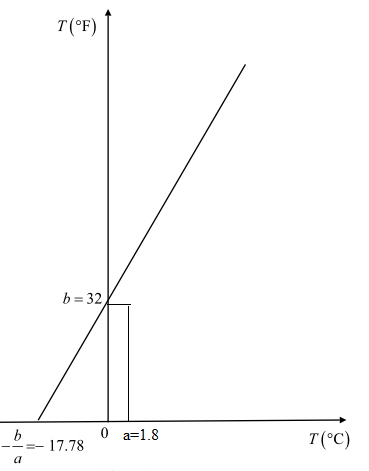
The relationship between the temperatures in Fahrenheit and Celsius scales satisfies the linear equation $T\left(°\text{F}\right)=aT\left(°\text{C}\right)+b$. (a) Using the given data, find the equation of the line relating the Fahrenheit and Celsius scales

(b) Sketch the graph of $T\left(°\text{F}\right)$ as a function of $T\left(°\text{C}\right)$, and clearly indicate a arid b on your graph.

(c) Using the graph obtained in part (b ), find the temperature interval in °C if the temperature is between 20°F and 80°F.