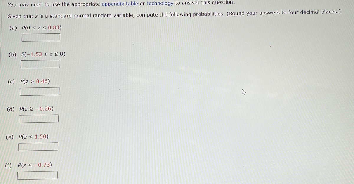
You may need to use the appropriate appendix table or technology to answer this question. Given that z is a standard normal random variable, compute the following probabilities. (Round your answers to four decimal places.) (a) P(0 ≤ z < 0.83) (b) P(-1.53 ≤ Z ≤ 0) (c) P(z > 0.46) (d) P(z ≥ -0.26) (e) P(z <1.50) (f) P(z≤ -0.73) W

If you add several normally distributed random numbers, the result is normally distributed, where the mean of the sum is the sum of the individual means, and the variance of the sum is the sum of the individual variances. (Remember that variance is the square of standard deviation.) This is a difficult result to prove mathematically, but it is easy to demonstrate with simulation. To do so, run a simulation where you add three normally distributed random numbers, each with mean 100 and standard deviation 10. Your single output variable should be the sum of these three numbers. Verify with @RISK that the distribution of this output is approximately normal with mean 300 and variance 300 (hence, standard deviation 300=17.32).

Dilberts Department Store is trying to determine how many Hanson T-shirts to order. Currently the shirts are sold for 21, but at later dates the shirts will be offered at a 10% discount, then a 20% discount, then a 40% discount, then a 50% discount, and finally a 60% discount. Demand at the full price of 21 is believed to be normally distributed with mean 1800 and standard deviation 360. Demand at various discounts is assumed to be a multiple of full-price demand. These multiples, for discounts of 10%, 20%, 40%, 50%, and 60% are, respectively, 0.4, 0.7, 1.1, 2, and 50. For example, if full-price demand is 2500, then at a 10% discount customers would be willing to buy 1000 T-shirts. The unit cost of purchasing T-shirts depends on the number of T-shirts ordered, as shown in the file P10_36.xlsx. Use simulation to determine how many T-shirts the company should order. Model the problem so that the company first orders some quantity of T-shirts, then discounts deeper and deeper, as necessary, to sell all of the shirts.

Suppose that a regional express delivery service company wants to estimate the cost of shipping a package (Y) as a function of cargo type, where cargo type includes the following possibilities: fragile, semifragile, and durable. Costs for 15 randomly chosen packages of approximately the same weight and same distance shipped, but of different cargo types, are provided in the file P13_16.xlsx. a. Estimate a regression equation using the given sample data, and interpret the estimated regression coefficients. b. According to the estimated regression equation, which cargo type is the most costly to ship? Which cargo type is the least costly to ship? c. How well does the estimated equation fit the given sample data? How might the fit be improved? d. Given the estimated regression equation, predict the cost of shipping a package with semifragile cargo.

When you use @RISKs correlation feature to generate correlated random numbers, how can you verify that they are correlated? Try the following. Use the RISKCORRMAT function to generate two normally distributed random numbers, each with mean 100 and standard deviation 10, and with correlation 0.7. To run a simulation, you need an output variable, so sum these two numbers and designate the sum as an output variable. Run the simulation with 1000 iterations and then click the Browse Results button to view the histogram of the output or either of the inputs. Then click the Scatterplot button below the histogram and choose another variable (an input or the output) for the scatterplot. Using this method, are the two inputs correlated as expected? Are the two inputs correlated with the output? If so, how?

An antique collector believes that the price received for a particular item increases with its age and with the number of bidders. The file P13_14.xlsx contains data on these three variables for 32 recently auctioned comparable items. Estimate a multiple regression equation using the given data. Interpret each of the estimated regression coefficients. Is the antique collector correct in believing that the price received for the item increases with its age and with the number of bidders? Interpret the standard error of estimate and the R-square value for these data.

Suppose you have invested 25% of your portfolio in four different stocks. The mean and standard deviation of the annual return on each stock are shown in the file P11_46.xlsx. The correlations between the annual returns on the four stocks are also shown in this file. a. What is the probability that your portfolios annual return will exceed 30%? b. What is the probability that your portfolio will lose money during the year?

Based on Babich (1992). Suppose that each week each of 300 families buys a gallon of orange juice from company A, B, or C. Let pA denote the probability that a gallon produced by company A is of unsatisfactory quality, and define pB and pC similarly for companies B and C. If the last gallon of juice purchased by a family is satisfactory, the next week they will purchase a gallon of juice from the same company. If the last gallon of juice purchased by a family is not satisfactory, the family will purchase a gallon from a competitor. Consider a week in which A families have purchased juice A, B families have purchased juice B, and C families have purchased juice C. Assume that families that switch brands during a period are allocated to the remaining brands in a manner that is proportional to the current market shares of the other brands. For example, if a customer switches from brand A, there is probability B/(B + C) that he will switch to brand B and probability C/(B + C) that he will switch to brand C. Suppose that the market is currently divided equally: 10,000 families for each of the three brands. a. After a year, what will the market share for each firm be? Assume pA = 0.10, pB = 0.15, and pC = 0.20. (Hint: You will need to use the RISKBINOMLAL function to see how many people switch from A and then use the RISKBENOMIAL function again to see how many switch from A to B and from A to C. However, if your model requires more RISKBINOMIAL functions than the number allowed in the academic version of @RISK, remember that you can instead use the BENOM.INV (or the old CRITBENOM) function to generate binomially distributed random numbers. This takes the form =BINOM.INV (ntrials, psuccess, RAND()).) b. Suppose a 1% increase in market share is worth 10,000 per week to company A. Company A believes that for a cost of 1 million per year it can cut the percentage of unsatisfactory juice cartons in half. Is this worthwhile? (Use the same values of pA, pB, and pC as in part a.)

In Example 11.2, the gamma distribution was used to model the skewness to the right of the lifetime distribution. Experiment to see whether the triangular distribution could have been used instead. Let its minimum value be 0, and choose its most likely and maximum values so that this triangular distribution has approximately the same mean and standard deviation as the gamma distribution in the example. (Use @RISKs Define Distributions window and trial and error to do this.) Then run the simulation and comment on similarities or differences between your outputs and the outputs in the example.

Management of a home appliance store would like to understand the growth pattern of the monthly sales of Blu-ray disc players over the past two years. Managers have recorded the relevant data in the file P13_33.xlsx. a. Create a scatterplot for these data. Comment on the observed behavior of monthly sales at this store over time. b. Estimate an appropriate regression equation to explain the variation of monthly sales over the given time period. Interpret the estimated regression coefficients. c. Analyze the estimated equations residuals. Do they suggest that the regression equation is adequate? If not, return to part b and revise your equation. Continue to revise the equation until the results are satisfactory.