
ENGR.ECONOMIC ANALYSIS
14th Edition
ISBN: 9780190931919
Author: NEWNAN
Publisher: Oxford University Press
expand_more
expand_more
format_list_bulleted
Question
The graph attached illustrates the Demand, Marginal Revenue, Marginal Costs, Average Total Costs and Average variable Cost curves for a firm in a perfectly competitive market.
- What is the Optimum level of the output for the firm and what is the maximum
price the firm can charge? How do you know? - At this price and output combination does the firm make economic profit of economic loss? Explain your answer.
- Calculate the economic profit or loss? Show your calculations.
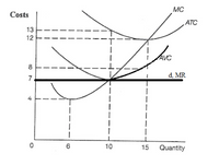
Transcribed Image Text:This graph illustrates various cost curves in microeconomics, ideal for an educational website explaining cost structures in a firm. The vertical axis represents costs, and the horizontal axis represents quantity.
Key elements of the graph:
1. **MC (Marginal Cost)**: This curve typically slopes upward, indicating that each additional unit of output costs more to produce than the previous one.
2. **ATC (Average Total Cost)**: This curve initially declines, reaches a minimum, and then slopes upward. It reflects the cost per unit of output, calculated by dividing total costs by the quantity produced.
3. **AVC (Average Variable Cost)**: This curve shows a U-shape, similar to the ATC but starts lower and meets the ATC at the minimum point of the ATC. It accounts for variable costs per unit of output.
4. **d, MR (Demand and Marginal Revenue)**: Represented as a horizontal line at a cost of 7. This line demonstrates a perfectly elastic demand, meaning the price remains constant regardless of quantity produced.
Key intersections:
- The intersection of the **MC** and **ATC** around a quantity of 10 indicates the minimum point of the ATC and is significant for determining the most efficient scale of production.
- The horizontal line at the cost of 7 also intersects where the MC, ATC, and AVC meet, representing the break-even point where the firm covers all costs but does not make a profit.
This graph is crucial for understanding how firms decide on production levels to maximize profit or minimize losses, emphasizing the importance of the marginal cost and its impact on overall firm strategy.
Expert Solution
This question has been solved!
Explore an expertly crafted, step-by-step solution for a thorough understanding of key concepts.
This is a popular solution
Trending nowThis is a popular solution!
Step by stepSolved in 2 steps

Knowledge Booster
Learn more about
Need a deep-dive on the concept behind this application? Look no further. Learn more about this topic, economics and related others by exploring similar questions and additional content below.Similar questions
- you've been learning about what makes a market perfectly competitive, how a firm in a perfectly competitive market makes profit-maximizing decisions, and how a perfectly competitive market moves towards equilibirium. But how applicable is this to real life? For this discussion, try to think of a market (for a product or service) that is perfectly competitive or very close to it. What characteristics of the market make it like perfect competition? Are there factors that keep it from being perfectly competitive? If so, what are they? How close do you think the firms in this market are to perfectly competitive firms in choosing equilibrium price and quantity?arrow_forwardThe table below provides revenue and cost information for a perfectly competitive firm producing computers. How much are total costs if 3 computers are produced? How much are total variable costs if 5 computers are produced? What is the price of a computer? What is the average revenue from producing computers? What is the marginal revenue of producing computers? Over what output range will firm earn economic profits?arrow_forwardWhen would a profit-maximizing firm shut down in the short run?arrow_forward
- Problem two Consider the total cost and total revenue given in the following table: Total Total Quantity cost Revenue 0 1 2 3 4 5 6 7 8 9 10 11 13 19 27 37 0 8 16 24 32 40 48 56 a) Calculate the profit for each quantity. How much should the firm produce to maximize profit? b) Calculate the marginal revenue and marginal cost for each quantity. Graph them. c) Can you tell whether this firm is in a competitive industry? If so, can you tell whether the industry is in a long-run equilibrium?arrow_forwardAssume the following regarding a firm in Perfect Competition: Market Demand = Qd 460-3P Market Supply = Qs = 9 P Each identical firm has: MC=4q ATC = 14 1. What price will the firm charge? Number 2. What is the firm's equilibrium quantity? Number 3. What is the firm's total cost? Number 4. What is the firm's total revenue? Number 5. What is the firm's profit or loss? (use a negative sign to indicate a loss) Number 6. Is the firm in a short-run or long-run situation? Click for Listarrow_forwardThe equations below correspond with questions #1 - 2 below and describe the costs of a profit maximizing, perfectly competitive firm (q = output): Total Costs TC = 300 if q = 0 Total Costs TC = 400 + 10q + 2q2 if q > 0 Marginal Cost MC = 10 + 4q if q> 0 What is the greatest possible profit that this firm would earn if the market price is set at $90? a. $1800 b. $100 c. $400 d. $1400 e. none of the abovearrow_forward
- What type of industry has the characteristics where there are many producers, they are able to differentiate their product, the barriers to entry are low, and a firm in the industry has the ability to manipulate price to a certain extent. What type of industry is this? Will this type of industry be able to enjoy profits in the long run? Why? Also is this firm producing at productivity and allocative efficiency? Why?arrow_forwardExplain how to determine a firm's cost of production and economic profitarrow_forwardPlease answer F and show steps for the grapharrow_forward
- A friend has just started up her own business. Her firm asks you how much to charge for her product to maximize profits. The demand schedule for it is given by the first two columns in the table below; its total costs are given in the third column. For each level of output, you can calculate total revenue, marginal revenue, average cost, and marginal cost. The profit-maximizing level of output can be found at the point where TR - TC is greatest, or where MR = MC, (or the last quantity where MR is still greater than MC.) What is the profit-maximizing level of output for her product? 40 How much will she earn in profits? 80 Price Quantity TC TR? MR? MC? $25.00 0 $130 $24.00 10 $275 $23.00 20 $435 $22.50 30 $610 $22.00 40 $800 $21.60 50 $1,005 $21.20 60 $1,225arrow_forwardIf marginal revenue is $9, how much output will the firm produce, and how much profit will it make? Show your calculations.arrow_forwardUse the following table to answer the next question. The table shows the total costs associated with varying levels of output produced by a perfectly competitive firm. Output 0 1 2 3 4 Total Cost $1,400 1,600 2,000 2,600 3,500 4,800 If the product sells for $800 a unit, the firm's profit-maximizing output isarrow_forward
arrow_back_ios
SEE MORE QUESTIONS
arrow_forward_ios
Recommended textbooks for you

 Principles of Economics (12th Edition)EconomicsISBN:9780134078779Author:Karl E. Case, Ray C. Fair, Sharon E. OsterPublisher:PEARSON
 Engineering Economy (17th Edition)EconomicsISBN:9780134870069Author:William G. Sullivan, Elin M. Wicks, C. Patrick KoellingPublisher:PEARSON
 Principles of Economics (MindTap Course List)EconomicsISBN:9781305585126Author:N. Gregory MankiwPublisher:Cengage Learning
 Managerial Economics: A Problem Solving ApproachEconomicsISBN:9781337106665Author:Luke M. Froeb, Brian T. McCann, Michael R. Ward, Mike ShorPublisher:Cengage Learning
 Managerial Economics & Business Strategy (Mcgraw-...EconomicsISBN:9781259290619Author:Michael Baye, Jeff PrincePublisher:McGraw-Hill Education


Principles of Economics (12th Edition)
Economics
ISBN:9780134078779
Author:Karl E. Case, Ray C. Fair, Sharon E. Oster
Publisher:PEARSON

Engineering Economy (17th Edition)
Economics
ISBN:9780134870069
Author:William G. Sullivan, Elin M. Wicks, C. Patrick Koelling
Publisher:PEARSON

Principles of Economics (MindTap Course List)
Economics
ISBN:9781305585126
Author:N. Gregory Mankiw
Publisher:Cengage Learning

Managerial Economics: A Problem Solving Approach
Economics
ISBN:9781337106665
Author:Luke M. Froeb, Brian T. McCann, Michael R. Ward, Mike Shor
Publisher:Cengage Learning

Managerial Economics & Business Strategy (Mcgraw-...
Economics
ISBN:9781259290619
Author:Michael Baye, Jeff Prince
Publisher:McGraw-Hill Education