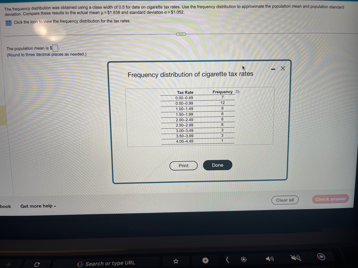
The frequency distribution was obtained using a class width of 0.5 for data on cigarette tax rates. Use the frequency distribution to approximate the population mean and population standard deviation. Compare these results to the actual mean μ= $1.638 and standard deviation o=$1.052. Click the icon to view the frequency distribution for the tax rates. The population mean is $ (Round to three decimal places as needed.)

The frequency distribution was obtained using a class width of 0.5 for data on cigarette tax rates. Use the frequency distribution to approximate the population mean and population standard deviation. Compare these results to the actual mean u= $1.885 and standard deviation o = $1.115. E Click the icon to view the frequency distribution for the tax rates. The population mean is S (Round to three decimal places as needed.)

In California, we need more rain to sustain the health of our natural environment, argriculture, and economic. A group of statistics students in Oxnard College recorded the amount of rain during 2016-2017 school year, measuring the intensity by the inches of rain, and the results were: Inches of Rain 2. 4 Frequency 4 4 3 1 3 The mean (T) rain intensity: inches (Please show your answer to 1 decimal place.) The median rain intensity: inches The mode rain intensity: inches (Please separate your answers by ',' in the bimodal situation. Enter DNE if there is no mode or if there are more than two modes.) Submit Question N 16 rch home ins prt sc delete 144

A recent Nielsen analysis found that the typical U.S. smartphone user is spending an average of 220 minutes per day using apps. We speculate that the average time spent using apps for Generation X smartphone users (aged 41-56 years) is less than the national average. The hypotheses are Ho: H = 220 minutes versus Ha: µ < 220 minutes. Summary results from R are provided. Summary Statistics Std. Dev (s) Mean Sample Size (n) 205 minutes 63.25 minutes 31

Please, find Arthematic Mean, Geomatric Mean, Harmonic Mean, Mode & Median of the given data. ASAP

The amount of caffeine in a sample of five-ounce servings of brewed coffee is shown in the histogram. Make a frequency distribution for the data. Then use the table to estimate the sample mean and the sample standard deviation of the data set. Click the icon to view the histogram. Complete the table. Round values to the nearest tenth as needed. Graph/chart f Midpoint x xf 70.5 Ay 30- 92.5 26 25- 114.5 136.5 20- 158.5 15- 12 Ef = Exf = 10- Find the mean of the data set. 5- X = (Round to the nearest tenth as needed.) 48.5 70.5 92.5 114.5 136.5 158.5 Complete the table. Round values to the nearest tenth as needed. Midpoint x (x-x)? (x-x)?f X-X 70.5 Print Done 92.5 114.5 136.5 158.5 (x-x)?r= ] of

The amount of caffeine in a sample of five-ounce servings of brewed coffee is shown in the histogram. Make a frequency distribution for the data. Then use the table to estimate the sample mean and the sample standard deviation of the data set. W Click the icon to view the histogram. .. Complete the table. Round values to the nearest tenth as needed. Graph/chart f Midpoint x xf 70.5 Ay 30- 25- 24 20- |14 15- 10- 17 5- X 48.5 70.5 92.5 114.5 136.5 158.5

Draw by hand or in Excel fully labelled curves on a common scale to represent two sets of scores where: b. Mean = 50, Standard Deviation = 2, Mean = 50, Standard Deviation = 5. CUA

Please help me solve this? Thanks

The coefficient of variation CV describes the standard deviation as a percent of the mean. Because it has no units, you can use the coefficient of variation to compare data with different units. Find the coefficient of variation for each sample data set. What can you conclude? Standard deviation CV = • 100% Mean E Click the icon to view the data sets. Data Table ..... CVneights = 71.2% (Round to the nearest tenth as needed.) Heights Weights 68 181 77 169 72 167 72 207 71 177 70 175 78 185 69 186 67 221 70 216 67 209 73 206