
MATLAB: An Introduction with Applications
6th Edition
ISBN: 9781119256830
Author: Amos Gilat
Publisher: John Wiley & Sons Inc
expand_more
expand_more
format_list_bulleted
Related questions
Question
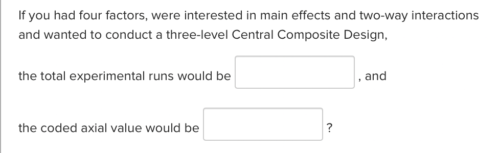

Transcribed Image Text:If you had four factors, were interested in main effects and two-way interactions
and wanted to conduct a three-level Central Composite Design,
the total experimental runs would be
the coded axial value would be
?
and
Expert Solution
This question has been solved!
Explore an expertly crafted, step-by-step solution for a thorough understanding of key concepts.

Step by stepSolved in 2 steps with 3 images

Knowledge Booster

Similar questions
- 4. The following output from R presents the results from computing a linear model. In our data example we are interested to study the relationship between students' academic performance api00 with variable enroll which is the number of students in the school. Call: Im (formula = api00 enroll, data = d) Residuals: мin 10 Median 30 Маx -285.50 -112.55 -6.70 95.06 389.15 Coefficients: Estimate Std. Error t value Pr(>|t|) (Intercept) 744.25141 15.93308 46.711 < 2e-16 *** enroll -0.19987 0.02985 -6.695 7.34e-11 *** --- Signif. codes: O ' *** ' 0.001 '**' 0.01 '*' 0.05 '.' 0.1 ' ' 1 Residual standard error: 135 on 398 degrees of freedom Multiple R-squared: 0.1012, Adjusted R-squared: F-statistic: 44.83 on 1 and 398 DF, p-value: 7.339e-11 0.09898arrow_forwardANSWER THE FOLLOWING QUESTION.arrow_forward1. Consider the following regression model: Fram Risk Score; = Bo + B1 × Health Insurance; + u¿ The Framingham Risk Score predicts 10-year risk of cardiovascular disease based on age, cholesterol levels, blood pressure, blood sugar, use of medication for high blood pressure, and smoking. A higher score means worse overall cardiovascular health. A researcher who collects data and regresses the Fram Risk Score against Health Insurance (= 1 if have insurance) finds that B, 2. Consider the following regression model: Class Average; = Bo + B1 x Office Hours; + u; Class Average is the students' average grade in the class at the end of the term and Office Hours is the number of office hours held by the instructor over the entire term. A researcher who collects data and regresses Class Average against Office Hours finds that, surprisingly, B V A V Aarrow_forward
- A study examined the eating habits of 20 children at a nursery school. The variables measured for each child included: calories (the number of calories eaten at lunch), time (the time in minutes spent eating lunch), and sex (male=1, female=0). A multiple linear regression model using Y = calories, X1 = time, and X2 = sex led to the following model: y=547.65-2.85x1+10.67x2 For two children who spend the same amount of time eating, one male and one female, which child is predicted to consume more calories and by how much?arrow_forwardBiologist Theodore Garland, Jr. studied the relationship between running speeds and morphology of 49 species of cursorial mammals (mammals adapted to or specialized for running). One of the relationships he investigated was maximal sprint speed in kilometers per hour and the ratio of metatarsal-to-femur length. A least-squares regression on the data he collected produces the equation ŷ = 37.67 + 33.18x %3D where x is metatarsal-to-femur ratio and ŷ is predicted maximal sprint speed in kilometers per hour. The standard error of the intercept is 5.69 and the standard error of the slope is 7.94. Construct an 80% confidence interval for the slope of the population regression line. Give your answers precise to at least two decimal places. Lower limit: Upper limit:arrow_forwardThe U.S. online grocery market is estimating sales worth approximately $29.7 billion by 2021. One of the biggest situational factors that influence the amount spent by a customer is the distance that that customer lives from its closest grocery store. Using the OLS method, the simple regression equation was estimated as: y = 40 + 3.5x. Find 1) the predicted amount a customer spends if they live 10 miles from the closest grocery store, as well as 2) the error amount. Note: the observed amount spent by a customer that lives 10 miles away is $85.50. a) $75.00, $10.50 Ob) $75.00, -$10.50 c) $73.00, $12.50 d) $73.00, -$12.50arrow_forward
- A well-known university is interested in how salary (in thousands of dollars) is predicted from years of service for faculty and administrative staff. Below are the estimated regression equations.Faculty (n = 170): ŷ = 60 + 1.1xAdmin. (n = 155): ŷ = 57 + 1.5x a) How much would a faculty member be earning after 5 years of service? b) In how many years will an administrator earn the same amount as in a)?arrow_forward)A county real estate appraiser wants to develop a statistical model to predict the appraised value of 3) houses in a section of the county called East Meadow. One of the many variables thought to be an important predictor of appraised value is the number of rooms in the house. Consequently, the appraiser decided to fit the simple linear regression model: E(u) = Bo + Bix, where y = appraised value of the house (in thousands of dollars) and x = number of rooms. Using data collected for a sample of n = 73 houses in Fast Meadow, the following results were obtained: y = 73.80 + 19.72x What are the properties of the least squares line, y = 73.80 + 19.72x? A) Average error of prediction is 0, and SSE is minimum. B) It will always be a statistically useful predictor of y. C) It is normal, mean 0, constant variance, and independent. D) All 73 of the sample y-values fall on the line.arrow_forward
arrow_back_ios
arrow_forward_ios
Recommended textbooks for you
- MATLAB: An Introduction with ApplicationsStatisticsISBN:9781119256830Author:Amos GilatPublisher:John Wiley & Sons Inc
 Probability and Statistics for Engineering and th...StatisticsISBN:9781305251809Author:Jay L. DevorePublisher:Cengage Learning
 Statistics for The Behavioral Sciences (MindTap C...StatisticsISBN:9781305504912Author:Frederick J Gravetter, Larry B. WallnauPublisher:Cengage Learning
  Elementary Statistics: Picturing the World (7th E...StatisticsISBN:9780134683416Author:Ron Larson, Betsy FarberPublisher:PEARSON
 The Basic Practice of StatisticsStatisticsISBN:9781319042578Author:David S. Moore, William I. Notz, Michael A. FlignerPublisher:W. H. Freeman
 Introduction to the Practice of StatisticsStatisticsISBN:9781319013387Author:David S. Moore, George P. McCabe, Bruce A. CraigPublisher:W. H. Freeman
MATLAB: An Introduction with Applications
Statistics
ISBN:9781119256830
Author:Amos Gilat
Publisher:John Wiley & Sons Inc
Probability and Statistics for Engineering and th...
Statistics
ISBN:9781305251809
Author:Jay L. Devore
Publisher:Cengage Learning
Statistics for The Behavioral Sciences (MindTap C...
Statistics
ISBN:9781305504912
Author:Frederick J Gravetter, Larry B. Wallnau
Publisher:Cengage Learning
Elementary Statistics: Picturing the World (7th E...
Statistics
ISBN:9780134683416
Author:Ron Larson, Betsy Farber
Publisher:PEARSON
The Basic Practice of Statistics
Statistics
ISBN:9781319042578
Author:David S. Moore, William I. Notz, Michael A. Fligner
Publisher:W. H. Freeman
Introduction to the Practice of Statistics
Statistics
ISBN:9781319013387
Author:David S. Moore, George P. McCabe, Bruce A. Craig
Publisher:W. H. Freeman