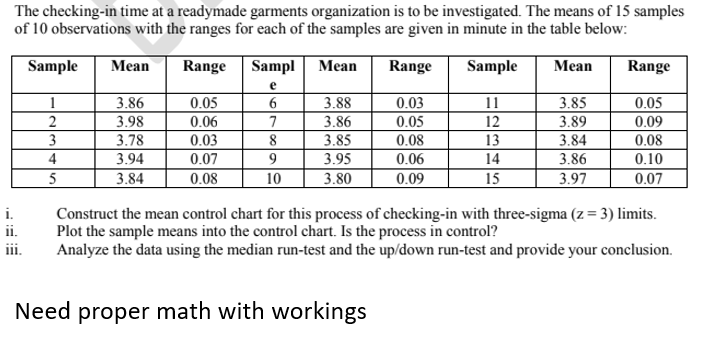
The checking-in time at a readymade garments organization is to be investigated. The means of 15 samplesof 10 observations with the ranges for each of the samples are given in minute in the table below:SampleМeanRangeSamplМeanRangeSampleМeanRangee3.883.8613.863.980.050.03113.850.0520.0670.05123.890.0933.780.0383.850.08133.840.0843.940.073.950.06143.860.1053.840.08103.800.09153.970.07Construct the mean control chart for this process of checking-in with three-sigma (z = 3) limits.Plot the sample means into the control chart. Is the process in control?Analyze the data using the median run-test and the up/down run-test and provide your conclusion.ii.Need proper math with workings

Answered: Image /qna-images/answer/b5e934d3-bc47-495e-909b-9d4285ba6ae3.jpg

Answered: of 10 observations with the ranges for…

MATLAB: An Introduction with Applications

6th Edition

ISBN:9781119256830

Author:Amos Gilat

Publisher:Amos Gilat

Chapter1: Starting With Matlab

Section: Chapter Questions

Problem 1P

See similar textbooks

Similar questions

The IQs of individuals form a normal distribution with mean = 100 and s = 15. A. What percentage of the population have IQs below 85? B. What percentage have IQs over 130? C. A college requires an IQ of 120 or more for entrance. From what percentage of the population must it draw its students? D. In a state with 400,000 high school seniors, how many meet the IQ requirement?
1/For the below frequency distribution table calculate all the below reequipments. Class Frequency 2-4 6-8 10-12 14-16 7 8 5 3 1. Medium -- 2. Mode -- 3. The Mean Deviation 4. Variance 5. Standard Deviation 6. Standardized Score
From the list below of the data being collected, identify which data would be considered variable data: Select ALL correct answers. Door closing speed at Honda Time before a call is answered at a call center Number of mistakes/miss-information given per call at a call center Percentage of medical bills with more than one defect Number of defects on one medical bill Weight of a golf ball Meal delivery time at a restaurant Number of orders with incorrect products per every 100 sampled at Amazon NEXT QUESTION From the list below of the data being collected, identify which data would be considered attribute data: Select ALL correct answers. Door closing speed at Honda Time before a call is answered at a call center Number of mistakes/miss-information given per call at a call center Percentage of medical bills with more than one defect Number of defects on one medical bill Weight of a golf ball Meal delivery time at a restaurant…
2. Shafts manufactured for use in optical storage devices have diameters that are normally distributed with mean u = 0.653 cm and standard deviation o = 0.002 cm. The specification for the shaft diameter is 0.650 + 0.005 cm. a. What proportion of the shafts manufactured by this process meet the specifications? b. The process mean can be adjusted through calibration. If the mean is set to
Identify the range, variance and standard deviation. show complete solutions
Four different paints are advertised as having the same drying time. To check the manufacturers' claims, five samples were tested for each of the paints. The time in minutes until the paint was dry enough for a second coat to be applied was recorded for each sample. The data obtained follow. Excel File: data16-21.xls Paint 3 Paint 4 133 150 143 142 137 135 136 140 131 153 a. Use a = 0.05 to test for any significant differences in mean drying time among the paints. If your answer is zero, enter "0". Lets define the dummy variables as follows: D1 20100 D2 0 0 1 D3 0 0 0 1 Paint 1 128 137 135 124 141 Paint 1234 Paint 2 144 133 142 146 130
To determine if their 1.50 inch steel handles are properly adjusted, Smith & Johnson Industries has decided to use an X-Chart which uses the range to estimate the variability in the sample. AnswerHow Step 3 of 7: What is the Lower Control Limit? Round your answer to three decimal places. Period obs1 obs2 obs3 obs4 obs5 1 1.46 1.50 1.46 1.53 1.55 1.54 1.45 1.50 1.54 1.52 1.49 1.53 1.47 1.51 1.47 1.49 1.53 5 1.54 1.50 1.47 1.46 1.54 1.53 1.46 1.51 1.52 1.49 1.46 1.55 1.45 1.47 1.53 1.53 1.50 1.52 1.45 1.49 1.53 1.48 1.53 1.47 1.49 JAWN - Select the Copy Table button to copy all values. To select an entire row or column, either click on the row or column header or use the S and arrow keys. To find the average of the selected cells, select the Average Values button. Copy Table Average Values The average of the selected cell(s) is 1.460. Copy Value 2 3 4 6789 22 10 1.49 11 1.52 1.52 O Control Chart 12 Table obs6 1.54 1.46 1.52 1.47 1.45 1.50 1.53 1.46 1.45 1.49 1.51 1.52 1.51 1.50 1.47 1.54…
Use Chebyshevs rule and the empirical rule to describe the distribution of this data set. Count the actual number of observations that fall within one, two, and three standard deviations of the mean if the data set and compare these counts with the description of the the data set I developed.
Look at the attached images. Explain and analyse for INR group A and B. Thank you!
Below are the SPSS results of a related (dependent) samples t-test. Use the SPSS results to answer Questions 5, 6, and 7. Paired Samples Statistics Mean N Std. Deviation Std. Error Mean Pair 1 Statistics Posttest 57.1250 40 16.73962 2.64677 Statistics Pretest 49.9250 40 15.09014 2.38596 Paired Samples Test Paired Differences t df Sig. (2-tailed) Mean Std. Deviation Std. Error Mean Pair 1 Statistics Posttest - Statistics Pretest 7.200 12.313 ( a ) ( b ) ( c ) .001 Find the mean of the differences ( and standard deviation of the differences (Sd). Replace “a,” “b,” and “c” in the table above with the correct values. Round to the third decimal place. Do you think there is a statistically significant difference between the pretest and posttest at the .05 level of significance?
Identify the measures of central tendency and dispersion requested for the sample below. f Relative f Cumulative relative f a. Mode 10 0.137 0.137 b. Median 1 14 0.192 0.329 C. Mean 11 0.151 0.479 d. Range 3 9. 0.123 0.603 е. Variance 0.110 0.151 4 8 0.712 Standard deviation 11 0.863 10 0.137 1.000 SUM 73 1.000
Help please

SEE MORE QUESTIONS

Recommended textbooks for you

MATLAB: An Introduction with Applications

Statistics

ISBN:

9781119256830

Author:

Amos Gilat

Publisher:

John Wiley & Sons Inc

Probability and Statistics for Engineering and th…

Statistics

ISBN:

9781305251809

Author:

Jay L. Devore

Publisher:

Cengage Learning

Statistics for The Behavioral Sciences (MindTap C…

Statistics

ISBN:

9781305504912

Author:

Frederick J Gravetter, Larry B. Wallnau

Publisher:

Cengage Learning

MATLAB: An Introduction with Applications

Statistics

ISBN:

9781119256830

Author:

Amos Gilat

Publisher:

John Wiley & Sons Inc

Probability and Statistics for Engineering and th…

Statistics

ISBN:

9781305251809

Author:

Jay L. Devore

Publisher:

Cengage Learning

Statistics for The Behavioral Sciences (MindTap C…

Statistics

ISBN:

9781305504912

Author:

Frederick J Gravetter, Larry B. Wallnau

Publisher:

Cengage Learning

Elementary Statistics: Picturing the World (7th E…

Statistics

ISBN:

9780134683416

Author:

Ron Larson, Betsy Farber

Publisher:

PEARSON

The Basic Practice of Statistics

Statistics

ISBN:

9781319042578

Author:

David S. Moore, William I. Notz, Michael A. Fligner

Publisher:

W. H. Freeman

Introduction to the Practice of Statistics

Statistics

ISBN:

9781319013387

Author:

David S. Moore, George P. McCabe, Bruce A. Craig

Publisher:

W. H. Freeman

SEE MORE TEXTBOOKS