
MATLAB: An Introduction with Applications
6th Edition
ISBN: 9781119256830
Author: Amos Gilat
Publisher: John Wiley & Sons Inc
expand_more
expand_more
format_list_bulleted
Related questions
Question
In every class, there are some students who speed through their tests while other students continue working on their tests until the very last second. To investigate whether these behaviours affeci students' scores, a researcher collected data on the amount of time students spend on a test and their grades from that test (N =
15). The researcher saved the results of their study to a file called hw6_exams. cv. Load the data into jamovi and answer the following questions.
1. Conduct a regression analysis predicting exam grade from time spent on the test. Paste the resulting model fit table and model coefficients table here . Make sure you include the F-test in the model fit table.
2. Paste an appropriate graph from jamovi. Make sure it includes a regression line .
3. What is the value of the test statistic for the overall model ?
4. What is the degrees of freedom for the overall model ?
5. What is the precise p-value for the overall model? Make sure you report the value to at least three decimal places.
6. Is the overall model significant ?
7. What is the R2 value for the overall model ? What does this R2 value mean in plain language ?
8. What do the results of the overall model mean?
9. What is the value of the test statistic for the predictor?
10. What is the precise p-value for the predictor ? Make sure you report the value to at least three decimal places.
11. Is the predictor significant ?
12. What is the value of the coefficient representing the predictor-outcome relationship ?
13. Interpret the value of this coefficient in plain language
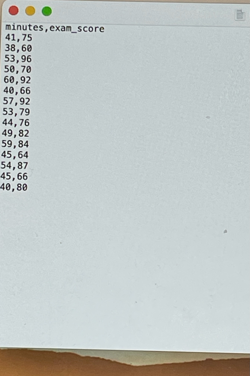

Transcribed Image Text:minutes, exam_score
41,75
38,60
53,96
50,70
60,92
40,66
57,92
53,79
44,76
49,82
59,84
45,64
54,87
45,66
40,80
Expert Solution
This question has been solved!
Explore an expertly crafted, step-by-step solution for a thorough understanding of key concepts.

Step by stepSolved in 3 steps with 1 images

Knowledge Booster

Similar questions
- A national study found that treating people appropriately for high blood pressure reduced their overall mortality by 20%. Treating people adequately for hypertension has been diffcult because it is estimated that 50% of hypertensives do not know they have high blood pressure, 50% of those who do know are inadequately treated by their physicians, and 50% who are appropriately treated fail to follow this treatment by taking the right number of pills. Answer the following questions ( please answer all the parts 1,2 and 3): 1) What is the probability that among 10 true hypertensives at least 50% are being treated appropriately and are complying with this treatment?2) What is the probability that at least 7 of the 10 hypertensives know they have high blood pressure? 3) If the preceding 50% rates were each reduced to 40% by a massive education program, then what effect would this change have on the overall mortality rate among true hypertensives; that is, would the mortality rate decrease…arrow_forwardSince muscle tension in the head region has been associated with tension headaches, a researcher reasoned that if the muscle tension could be changed, perhaps the headaches would also be changed. The researcher designed an experiment in which nine subjects with tension headaches participated. The subjects kept daily logs of the number of headaches they experienced during a 2-week baseline period. Then the researcher trained them to change their muscle tension in the head region, using a biofeedback device. For this experiment, the biofeedback device was connected to a muscle in the forehead region. The device indicated the subject's amount of tension in the muscle to which it was attached and helped them achieve low tension levels. After 6 weeks of training, during which the subjects became successful at maintaining low muscle tension, they again kept a 2-week log of the number of headaches experienced. The following are the number of headaches recorded during each 2-week period.…arrow_forwardSeveral states have argued that the 65-mph speed limit has no justification and have refused to enforce it. The federal Department of Transportation (DOT) believes that the 65-mph limit saves lives. To illustrate its contention, the department regressed the number of traffic fatalities (Y) last year in a state on the state’s population (X1), the number of days of snow cover (X2), and the average speed of all cars (X3). The results are shown below. Table 10: Model Summary Model R R Square Adjusted R Square Std. Error of the Estimate 1 .821 a .780 .613 3.258 a. Predictors: (Constant), population, days of snow, average speed Table 11: Coefficients Coefficientsa Model Unstandardized Coefficients Standardized Coefficients t Sig. B Std. Error Beta 1 (Constant) 1.4 2.957 .473 .584 Population .00029 .00003 .0034 9.667 .000 Days of Snow 2.4 .62 .759 3.871 .000 Average Speed 10.3 1.1…arrow_forward
- Mr. Palmer, has been teaching beginners how to fix their stroke for the last 10 years. The mean golfing score for all past students who learned with Mr. Palmer is 79. This golfing cycle, he tried a new teaching method using simulations instead of real-world golf. He then had 15 of his students that used his new method take a golfing test. Enter the data into SPSS. Use this dataset to answer this question: did Mr. Palmer’s students perform better on the golfing test using the new method as compared to the traditional teaching technique? 1. From the output, report the test statistic and the probability (obtained p-value, called “sig” in the output). Remember to include degrees of freedom when you report t-values. 2. Will you reject or fail to reject the null based on the SPSS output (Remember to use numbers from the output only to make your statistical conclusion. If you use a critical t, you will get no points.).arrow_forwardThe website Data USA stated that in 2016, Texas had the lowest number of adults with a serious mental illness with an average of M=3.26% of the population affected. The state of Texas wants to test if they have a significantly decreased number of mental illness patients compared with the states with the (n=8) highest level of mental illness found. In 2016 the following states had the highest level of adult patients with mental illness: Arkansas= 5.45%, Montana=5.34%, Vermont=5.32%, Oregon=5.19%, Utah=5.2%, Ohio=5.13, Kentucky=5.25% West Virginia=5.18%. The alpha level for the study was set to α=.05 for the criteria. a. State the hypotheses of the study. b. Find the critical t value for this study c. Compute the one-sample t test. (Again calculate sample SD or s - and get SEM before calculating t.) d. Compute the Cohen's d for the data (even if not significant) e. State the results - is the sample significantly higher? Do you reject the null hypothesis? Report the t test results in APA…arrow_forwardPeople gain weight when they take in more energy from food than they expend. Researchers wanted to investigate the link between obesity and energy spent on daily activity. Choose 20 healthy volunteers who don't exercise. Deliberately choose 10 who are lean and 10 who are mildly obese but still healthy. Attach sensors that monitor the subjects' every move for 10 days. The table below presents data on the time (in minutes per day) that the subjects spent standing or walking, sitting, and lying down. Is there a significant difference between the mean times the two groups spend lying down? Let ?1 be the mean time spent lying down by the lean group, and ?2 be the mean time for the obese group. Time (minutes per day) spent in three different postures by leanand obese subjects Group Subject Stand/Walk Sit Lie Lean 1 509.100 366.300 554.500 Lean 2 603.925 374.512 452.650 Lean 3 322.212 580.138 533.362 Lean 4 581.644 362.144 489.269 Lean 5…arrow_forward
- Elaine is interested in determining if men are more satisfied in their jobs than women in the healthcare industry. She administers a job satisfaction questionnaire to 20 men and 20 women working in hospital administration. Her grouping variable is gender and dependent variable is job satisfaction. The job satisfaction scale consists of 8 items measured using a 5-point rating scale. A higher score on this scale would indicate high job satisfaction. The maximum score that can be obtained on the scale is 40. We can assume that job satisfaction scores are normally distributed. Use the appropriate T test with a significance level of 0.05 to test the hypothesis. Research Question Do the mean job satisfaction scores differ for men and women working in the hospital administration department? Hypothesis The mean job satisfaction scores do not differ for men and women working in the hospital administration department. Compute an independent sample t test on these data. Report…arrow_forwardSeveral states have argued that the 65-mph speed limit has no justification and have refused to enforce it. The federal Department of Transportation (DOT) believes that the 65-mph limit saves lives. To illustrate its contention, the department regressed the number of traffic fatalities (Y) last year in a state on the state’s population (X1), the number of days of snow cover (X2), and the average speed of all cars (X3). The results are shown below. Table 10: Model Summary Model R R Square Adjusted R Square Std. Error of the Estimate 1 .821 a .780 .613 3.258 a. Predictors: (Constant), population, days of snow, average speed Table 11: Coefficients Coefficientsa Model Unstandardized Coefficients Standardized Coefficients t Sig. B Std. Error Beta 1 (Constant) 1.4 2.957 .473 .584 Population .00029 .00003 .0034 9.667 .000 Days of Snow 2.4 .62 .759 3.871 .000 Average Speed 10.3 1.1…arrow_forwardIn West Texas, water is extremely important. The following data represent pH levels in ground water for a random sample of 102 West Texas wells. A pH less than 7 is acidic and a pH above 7 is alkaline. Scanning the data, you can see that water in this region tends to be hard (alkaline). Too high a pH means the water is unusable or needs expensive treatment to make it usable†. These data are also available for download at the Companion Sites for this text. For convenience, the data are presented in increasing order.arrow_forward
arrow_back_ios
arrow_forward_ios
Recommended textbooks for you
- MATLAB: An Introduction with ApplicationsStatisticsISBN:9781119256830Author:Amos GilatPublisher:John Wiley & Sons Inc
 Probability and Statistics for Engineering and th...StatisticsISBN:9781305251809Author:Jay L. DevorePublisher:Cengage Learning
 Statistics for The Behavioral Sciences (MindTap C...StatisticsISBN:9781305504912Author:Frederick J Gravetter, Larry B. WallnauPublisher:Cengage Learning
  Elementary Statistics: Picturing the World (7th E...StatisticsISBN:9780134683416Author:Ron Larson, Betsy FarberPublisher:PEARSON
 The Basic Practice of StatisticsStatisticsISBN:9781319042578Author:David S. Moore, William I. Notz, Michael A. FlignerPublisher:W. H. Freeman
 Introduction to the Practice of StatisticsStatisticsISBN:9781319013387Author:David S. Moore, George P. McCabe, Bruce A. CraigPublisher:W. H. Freeman
MATLAB: An Introduction with Applications
Statistics
ISBN:9781119256830
Author:Amos Gilat
Publisher:John Wiley & Sons Inc
Probability and Statistics for Engineering and th...
Statistics
ISBN:9781305251809
Author:Jay L. Devore
Publisher:Cengage Learning
Statistics for The Behavioral Sciences (MindTap C...
Statistics
ISBN:9781305504912
Author:Frederick J Gravetter, Larry B. Wallnau
Publisher:Cengage Learning
Elementary Statistics: Picturing the World (7th E...
Statistics
ISBN:9780134683416
Author:Ron Larson, Betsy Farber
Publisher:PEARSON
The Basic Practice of Statistics
Statistics
ISBN:9781319042578
Author:David S. Moore, William I. Notz, Michael A. Fligner
Publisher:W. H. Freeman
Introduction to the Practice of Statistics
Statistics
ISBN:9781319013387
Author:David S. Moore, George P. McCabe, Bruce A. Craig
Publisher:W. H. Freeman