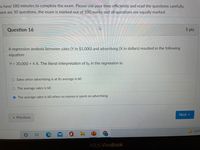
have 180 minutes to complete the exam. Please use your time efficiently and read the questions carefully. re are 30 questions, the exam is marked out of 100 marks and all questions are equally marked. Question 16 1 pts A regression analysis between sales (Y in $1,000) and advertising (X in dollars) resulted in the following equation Y = 30,000 + 4 X. The literal interpretation of bo in the regression is: O Sales when advertising is at its average is b0 The average sales is bo O The average sales is b0 when no money is spent on advertising Next « Previous ASUS VivoBook

You are interested in how the number of hours a high school student has to work in an outside job has on their GPA. In your regression you want to control for high school standing and so you run the following regression: GPA = 3.4 0.03 * HrsWrk - 0.7 * Frosh - 0.3 * Soph +0.1 * Junior (1.1) (0.013) (0.23) (0.14) (0.08) where HrsWrk is the number of hours the student works per week, and Frosh, Soph, and Junior are dummy variables for the student's class standing. a) If you include a dummy variable for seniors, that would cause a Hint: type one word in each blank. For the rest of questions, type a number in one decimal place. b) The expected GPA of a Sophomore who works 10 hours per week is c) The expected GPA of a Senior who works 10 hours per week is d) If Dom and Sarah work the same number of hours per week, but Dom is a Junior and Sarah is a Freshman. Dom is expected to have a higher GPA than Sarah. e) Suppose you rewrite the regression as: problem. GPA = ₁HrsWrk + ß2Frosh + B2Soph +…

Please help me with both the question. Answer there are incorrect

Help!