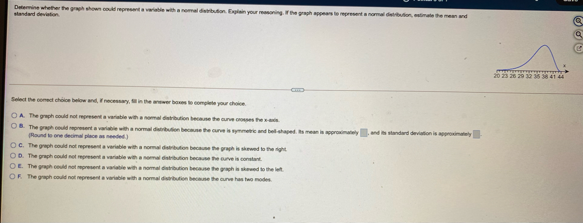
Determine whether the graph shown could represent a variable with a nomal distribution. Explain your reasoning. If the graph appears to represent a normal distribution, estimate the mean and standard deviation. 20 23 26 29 32 35 38 41 44 Select the corect chóice below and, if necessary, fill in the answer boxes to complete your choice. O A. The graph could not represent a variable with a normal distribution because the curve crosses the x-axis. O B. The graph could represent a variable with (Round to one decimal place as needed.) normal distribution because the curve is symmetric and bell-shaped. Its mean is approximately , and its standard deviation is approximately. O C. The graph could not represent a variable with a normal distribution because the graph is skewed to the right O D. The graph could not represent a variable with a normal distribution because the curve is constant. OE. The graph could not represent a variable with a normal distribution because the graph is skewed to the left. OF. The graph could not represent a variable with a normal distribution because the curve has two modes.

Dont copy the question. Answer only  Letter of the correct answer and explanation only if you want to explain .

Suppose that you are using independent samples to compare two population proportions. Fill in the blanks. a. The mean of all possible differences between the two sample proportions equals the_______.b. For large samples, the possible differences between the two samplel proportions have approximately a_________distribution.

Refer to the data set in the accompanying table. Assume that the paired sample data is a simple random sample and the differences have a distribution that is approximately normal. Use a significance level of 0.05 to test for a difference between the weights of discarded paper (in pounds) and weights of discarded plastic (in pounds). E Click the icon to view the data. In this example, Hg is the mean value of the differences d for the population of all pairs of data, where each individual difference d is defined as the weight of discarded paper minus the weight of discarded plastic for a household. What are the null and alternative hypotheses for the hypothesis test? O A. Ho: Ha = 0 H,: Ha #0 O B. Ho: Ha #0 H1: Hd =0 O C. Ho: Ha #0 O D. Ho: Ha = 0 H1: Hd 0