
ENGR.ECONOMIC ANALYSIS
14th Edition
ISBN: 9780190931919
Author: NEWNAN
Publisher: Oxford University Press
expand_more
expand_more
format_list_bulleted
Question
7. Short-run supply and long-run equilibrium
Consider the competitive market for steel. Assume that, regardless of how many firms are in the industry, every firm in the industry is identical and faces the marginal cost (MC), average total cost (ATC), and average variable cost (AVC) curves shown on the following graph.
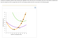
Transcribed Image Text:Consider the competitive market for steel. Assume that, regardless of how many firms are in the industry, every firm in the industry is identical and
faces the marginal cost (MC), average total cost (ATC), and average variable cost (AVC) curves shown on the following graph.
80
72
64
56
48
ATC
40
32
24
AVC
16
MC O
4
12
16
20
24
28
32
36
40
QUANTITY (Thousands of tons)
COSTS (Dollars per ton)
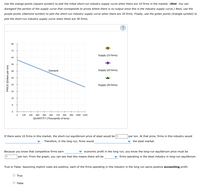
Transcribed Image Text:Use the orange points (square symbol) to plot the initial short-run industry supply curve when there are 10 firms in the market. (Hint: You can
disregard the portion of the supply curve that corresponds to prices where there is no output since this is the industry supply curve.) Next, use the
purple points (diamond symbol) to plot the short-run industry supply curve when there are 20 firms. Finally, use the green points (triangle symbol) to
plot the short-run industry supply curve when there are 30 firms.
80
72
Supply (10 firms)
64
56
48
Demand
Supply (20 firms)
40
32
Supply (30 firms)
24
16
120
240
360
480
600
720
B40
960
10B0 1200
QUANTITY (Thousands of tons)
If there were 10 firms in this market, the short-run equilibrium price of steel would be $
. Therefore, in the long run, firms would
|per ton. At that price, firms in this industry would
the steel market.
Because you know that competitive firms earn
economic profit in the long run, you know the long-run equilibrium price must be
24
per ton. From the graph, you can see that this means there will be
firms operating in the steel industry in long-run equilibrium.
True or False: Assuming implicit costs are positive, each of the firms operating in this industry in the long run earns positive accounting profit.
True
O False
PRICE (Dollars per ton)
Expert Solution
This question has been solved!
Explore an expertly crafted, step-by-step solution for a thorough understanding of key concepts.
This is a popular solution
Trending nowThis is a popular solution!
Step by stepSolved in 3 steps with 1 images

Knowledge Booster
Learn more about
Need a deep-dive on the concept behind this application? Look no further. Learn more about this topic, economics and related others by exploring similar questions and additional content below.Similar questions
- Consider the perfectly competitive market for steel. Assume that, regardless of how many firms are in the industry, every firm in the industry is identical and faces the marginal cost (MC), average total cost (ATC), and average variable cost (AVC) curves shown on the following graph. COSTS (Dollars per ton) PRICE (Dollars per ton) 100 90 80 70 20 100 10 90 0 80 70 10 0 0 The following diagram shows the market demand for steel. MC 5 0 123 ATC 0 ♫ Use the orange points (square symbol) to plot the initial short-run industry supply curve when there are 20 firms in the market. (Hint: You can disregard the portion of the supply curve that corresponds to prices where there is no output since this is the industry supply curve.) Next, use the purple points (diamond symbol) to plot the short-run industry supply curve when there are 30 firms. Finally, use the green points (triangle symbol) to plot the short-run industry supply curve when there are 40 firms. AVC 0 10 15 20 25 30 35 QUANTITY…arrow_forwardThe graph below shows the marginal cost (MC), average variable cost (AVC), and average total cost (ATC) curves for a firm in a competitive market. These curves imply a short-run supply curve that has two distinct parts. One part, not shown, lies along the vertical axis (quantity-0); this represents a condition of production shutdown. Where is the other part? Use the straight-line tool to drawit. To refer to the graphing tutorial for this question type, please click here Price and cost 18 15 14 13 12 10 19/21 SUBMIT ANSWER 13 OF 21 QUESTIONS C OMPLETED 28 MacBook Pro 금□ F7 F8 F9 F1o F2 F3 F5arrow_forwardThe blue curve on the following graph represents the demand curve facing a firm that can set its own prices. Use the graph input tool to help you answer the following questions. You will not be scored on any changes you make to this graph. Note: Once you enter a value in a white field, the graph and any corresponding amounts in each grey field will change accordingly. PRICE (Dollars per unit) 100 TOTAL REVENUE (Dollars) 90 80 20 10 0 1250 1125 1000 875 750 625 500 On the previous graph, change the number found in the Quantity Demanded field to determine the prices that correspond to the production of 0, 10, 20, 25, 30, 40, or 50 units of output. Calculate the total revenue for each of these production levels. Then, on the following graph, use the green points (triangle symbol) to plot the results. 375 250 125 + 0 0 0 Demand 5 10 15 20 25 30 35 40 45 50 QUANTITY (Units) + 5 20 10 15 25 30 35 QUANTITY (Number of units) 40 Graph Input Tool Market for Goods 45 50 Quantity Demanded (Units)…arrow_forward
- Firm Profit, Loss, and Shut Down Based upon the graph, answer the following questions: 1) What is the production level that will maximize the profit for the firm? 2) What is the profit-maximizing price the firm will charge? 3) Will the firm incur an economic gain or economic loss? 4) What will the dollar amount of economic gain or economic loss be? 5) What will be the price and quantity where the firm will shut down?arrow_forwardSuppose there are 7 firms in this industry, each of which has the cost curves previously shown. On the following graph, use the orange points (square symbol) to plot points along the portion of the industry's short-run supply curve that corresponds to prices where there is positive output. (Note: For the graphing tool to grade correctly, you must plot these points in order from left to right, starting with the point closest to the origin. You are given more points to plot than you need.) Next, place the black point (plus symbol) on the graph to indicate the short-run equilibrium price and quantity in this market. Note: Dashed drop lines will automatically extend to both axes. PRICE (Dorper stack ༞ ་ ་ ༞ སྠཽ བྷ བྷ * “ 100 20 10 Demand 0 0 70 140 210 200 250 420 490 500 430 700 QUANTITY (That of pack) ---- Industry's Short-Hun Supply + Equilibrium At the current short-run market price, firms will in the short run. In the long run,arrow_forwardShort-run supply and long-run equilibrium Consider the competitive market for titanium. Assume that, regardless of how many firms are in the industry, every firm in the industry is identical and faces the marginal cost (MC), average total cost (ATC), and average variable cost (AVC) curves shown on the following graph. Note:- Do not provide handwritten solution. Maintain accuracy and quality in your answer. Take care of plagiarism.Answer completely.You will get up vote for sure.arrow_forward
- The following graph plots daily cost curves for a firm operating in the competitive market for demin overalls. Hint: Once you have positioned the rectangle on the graph, select a point to observe its coordinates. PRICE (Dollars per overalls) 50 10 10 5 0 MC 2 ATC 8 18 QUANTITY (Thousands of overallises per day) AVC 10 20 Profit or Loss In the short run, given a market price equal to $15 per overalls, the firm should produce a daily quantity of On the preceding graph, use the blue rectangle (circle symbols) to fill in the area that represents profit or loss of the firm given the market price of $15 and the quantity of production from your previous answer. Note: In the following question, enter a positive number regardless of whether the firm earns a profit or incurs a loss. The rectangular area represents a short-run thousand per day for the firm. $ overallses.arrow_forward17th Assignment Consider a representative firm with total costs of TC = 16 + 1/Q ^ 2 (and a marginal cost of Q, MC = 1/2 * Q ) The market demand curve is given by P = 10 - 1/A * C and the starting market price is $2. 1) Graph the starting scenario using comparative statics. 2) Calculate any profit or loss. Why is this not a long run equilibrium? 3) What happens in order to transition to the long run? 4) Graph the long run equilibrium using comparative statics. 5) How many firms are in the market in the long run?.arrow_forward100 90 90 00 80 COSTS (Dollars) 70 70 00 60 50 40 30 20 10 ATC AVC MC 0 0 5 10 15 20 25 30 QUANTITY (Thousands of snapbacks) 35 35 40 45 50 For every price level given in the following table, use the graph to determine the profit-maximizing quantity of snapbacks for the firm. Further, select whether the firm will choose to produce, shut down, or be indifferent between the two in the short run. (Assume that when price exactly equals average variable cost, the firm is indifferent between producing zero snapbacks and the profit-maximizing quantity of snapbacks.) Lastly, determine whether the firm will earn a profit, incur a loss, or break even at each price. Price (Dollars per snapback) 10 20 32 40 50 60 Quantity (Snapbacks) Produce or Shut Down? Profit or Loss?arrow_forward
- Suppose the market for beans is perfectly competitive. The average total cost and marginal cost of growing beans in the long run for an individual farmer are illustrated in the graph to the right. According to the graph, the long run equilibrium price for beans is $ per box. (Enter a numeric response using a real number rounded to two decimal places.) C Price and cost (dollars per box) 10- 9- 00 N 1 0 10 MC 20 30 40 50 60 70 80 Quantity of beans (boxes per week) ATC 90 100 Narrow_forward7. Short-run supply and long-run equilibrium Consider the competitive market for rhenium. Assume that no matter how many firms operate in the industry, every firm is identical and faces the same marginal cost (MC), average total cost (ATC), and average variable cost (AVC) curves plotted in the following graph. COSTS (Dollars per pound) 100 90 80 70 60 40 20 10 + 0 + 0 MC + 5 ATC AVC D 0 10 15 20 25 30 35 QUANTITY (Thousands of pounds) 40 + 45 50 ?arrow_forwardConsider the perfectly competitive market for titanium. Assume that, regardless of how many firms are in the industry, every firm in the industry is identical and faces the marginal cost ( MCMC ), average total cost ( ATCATC ), and average variable cost ( AVCAVC ) curves shown on the following grapharrow_forward
arrow_back_ios
SEE MORE QUESTIONS
arrow_forward_ios
Recommended textbooks for you

 Principles of Economics (12th Edition)EconomicsISBN:9780134078779Author:Karl E. Case, Ray C. Fair, Sharon E. OsterPublisher:PEARSON
 Engineering Economy (17th Edition)EconomicsISBN:9780134870069Author:William G. Sullivan, Elin M. Wicks, C. Patrick KoellingPublisher:PEARSON
 Principles of Economics (MindTap Course List)EconomicsISBN:9781305585126Author:N. Gregory MankiwPublisher:Cengage Learning
 Managerial Economics: A Problem Solving ApproachEconomicsISBN:9781337106665Author:Luke M. Froeb, Brian T. McCann, Michael R. Ward, Mike ShorPublisher:Cengage Learning
 Managerial Economics & Business Strategy (Mcgraw-...EconomicsISBN:9781259290619Author:Michael Baye, Jeff PrincePublisher:McGraw-Hill Education


Principles of Economics (12th Edition)
Economics
ISBN:9780134078779
Author:Karl E. Case, Ray C. Fair, Sharon E. Oster
Publisher:PEARSON

Engineering Economy (17th Edition)
Economics
ISBN:9780134870069
Author:William G. Sullivan, Elin M. Wicks, C. Patrick Koelling
Publisher:PEARSON

Principles of Economics (MindTap Course List)
Economics
ISBN:9781305585126
Author:N. Gregory Mankiw
Publisher:Cengage Learning

Managerial Economics: A Problem Solving Approach
Economics
ISBN:9781337106665
Author:Luke M. Froeb, Brian T. McCann, Michael R. Ward, Mike Shor
Publisher:Cengage Learning

Managerial Economics & Business Strategy (Mcgraw-...
Economics
ISBN:9781259290619
Author:Michael Baye, Jeff Prince
Publisher:McGraw-Hill Education