
MATLAB: An Introduction with Applications
6th Edition
ISBN: 9781119256830
Author: Amos Gilat
Publisher: John Wiley & Sons Inc
expand_more
expand_more
format_list_bulleted
Related questions
Topic Video
Question

Transcribed Image Text:erences
Mailings
Review
View
Help
Aa A
AaBbCcL AaBbC AaBbCc AaBbCcl AaBbCcD AABBC
- A
Emphasis
Heading 1
1 Normal
Strong
Subtitle
Title
Paragraph
Styles
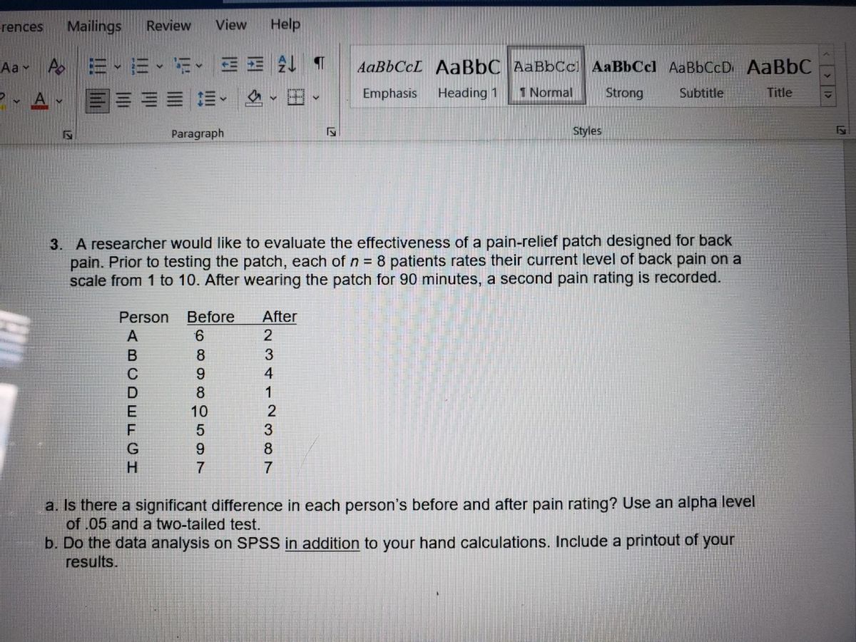
3. A researcher would like to evaluate the effectiveness of a pain-relief patch designed for back
pain. Prior to testing the patch, each of n = 8 patients rates their current level of back pain on a
scale from 1 to 10. After wearing the patch for 90 minutes, a second pain rating is recorded.
Person
Before
After
6.
8
C
6.
8.
10
9.
7
a. Is there a significant difference in each person's before and after pain rating? Use an alpha level
of .05 and a two-tailed test.
b. Do the data analysis on SPSS in addition to your hand calculations. Include a printout of your
results.
23412387
Expert Solution
This question has been solved!
Explore an expertly crafted, step-by-step solution for a thorough understanding of key concepts.

Step by stepSolved in 3 steps with 1 images

Knowledge Booster


Learn more about
Need a deep-dive on the concept behind this application? Look no further. Learn more about this topic, statistics and related others by exploring similar questions and additional content below.Similar questions
- Answer question 10 and 11 onlyarrow_forwardPrehistoric pottery vessels are usually found as sherds (broken pieces) and are carefully reconstructed if enough sherds can be found. Information taken from Mimbres Mogollon Archaeology by A. I. Woosley and A. J. McIntyre (University of New Mexico Press) provides data relating x = body diameter in centimeters and y = height in centimeters of prehistoric vessels reconstructed from sherds found at a prehistoric site. The following Minitab printout provides an analysis of the data. Predictor Coef SE Coef T P Constant -0.212 2.429 -0.09 0.929 Diameter 0.7527 0.1686 5.33 0.013 S = 4.16190 R-Sq = 81.2% (c) The formula for the margin of error E for a c% confidence interval for the slope ? can be written as E = tc(SE Coef). The Minitab display is based on n = 12 data pairs. Find the critical value tc for a 90% confidence interval in the relevant table. Then find a 90% confidence interval for the population slope ?. (Use 3 decimal places.) tc lower limit upper…arrow_forwardA study by Judge and Cable (2010) suggests that there is a positive relationship between weight and income for a group of men. The following data is similar to what was collected in the study. To simplify the weight variable, the men are categorized into five categories that measure actual weight relative to height from 1=thinnest to 5=heaviest. Income is recorded as thousands earned annually. Weight (X) Income (Y) 4 151 5 88 3 52 2 73 1 49 3 92 1 56 5 143 а. Calculate the Pearson correlation for these data. b. Is the correlation statistically significant? Use a two-tailed test with a=.05.arrow_forward
- Part e & d pleasearrow_forwardMaintaining your balance may get harder as you grow older. A study was conducted to see how steady the elderly are on their feet. They had a random sample of subjects stand on a force platform and have them react to a noise. The force platform then measured how much they swayed forward and backward, and the data are in the table below. Do the data show that the mean elderly sway measurement is higher than the mean forward sway of younger people, which is 18.125 mm? Test at the 1% level. forward sway in mm 34 30 31 34 24 25 22 33 33 17 19 29 30 31 24 33 27 26 26 30 17 17 15 41 48 34 15 36 20 9 34 12 13 34 14 29 39 33 11 20 25 29 23 27 P: Parameter What is the correct parameter symbol for this problem? What is the wording of the parameter in the context of this problem? H: Hypotheses Fill in the correct null and alternative hypotheses: H0:H0:…arrow_forwardWould someone familiar with SPSS be able to help with sub-question d please?arrow_forward
- A study by Judge and Cable (2010) suggests that there is a positive relationship between weight and income for a group of men. The following data is similar to what was collected in the study. To simplify the weight variable, the men are categorized into five categories that measure actual weight relative to height from 1=thinnest to 5=heaviest. Income is recorded as thousands earned annually. Weight (X) Income (Y) 4 151 5 88 3 52 2 73 1 49 3 92 1 56 5 143 a. Calculate the Pearson correlation for these data. b. Is the correlation statistically significant? Use a two-tailed test with a=.05.arrow_forwardPls show work so I can understandarrow_forwardAttachedarrow_forward
- Part 1 of 4 Does the length of a surgery patient's stay in the hospital depend on the length of time the operation took? The table below gives the operative time (in hours) and the length of the hospital stay (in days) for 10 patients. (Comma separated lists of the data are also provided below the table to ease in copying the data to R.) Operative Time (x) Length of Hospital Stay (y) 5 13 13 12 12 14 17 4 12 3 12 7 15 3 x: 5, 5, 5, 2, 6, 5, 4, 3, 7, 3 y: 13, 13, 12, 12, 14, 17, 12, 12, 15, 7 Conduct a hypothesis test with a 5% level of significance to determine whether or not the operative time and the length of a patient's hospital stay are correlated. Step 1: State the null and alternative hypotheses. Ho:p = test.) (So we will be performing a two-tailed O Rost to forumarrow_forwardAccording to the CDC, cholesterol levels can be reduced by following a healthy diet, getting regular exercise, and reducing the amount of alcohol consumed on a weekly basis. One method of monitoring overall cholesterol levels is to calculate your cholesterol ratio (LDL/HDL), in general a cholesterol ratio between 3.5 and 5.0 is considered to be healthy for most adults. Suppose you are a clinical researcher testing the effects of these lifestyle changes on patient cholesterol levels. In order to determine if following these guidelines helps to reduce overall cholesterol, a total of 18 participants (N = 18) with moderate to high cholesterol ratios (i.e., 3.91 to > 5.0) were recruited for a healthy lifestyle study and their cholesterol ratio was calculated three times over a six week period: Week 0 (baseline), Week 3, and Week 6. Using the variables "Week 0", "Week 3", and "Week 6" in the data set, conduct a One-Way, Within Subjects (AKA Repeated Measures) ANOVA, at α = 0.05, to see…arrow_forwardAccording to the CDC, cholesterol levels can be reduced by following a healthy diet, getting regular exercise, and reducing the amount of alcohol consumed on a weekly basis. One method of monitoring overall cholesterol levels is to calculate your cholesterol ratio (LDL/HDL), in general a cholesterol ratio between 3.5 and 5.0 is considered to be healthy for most adults. Suppose you are a clinical researcher testing the effects of these lifestyle changes on patient cholesterol levels. In order to determine if following these guidelines helps to reduce overall cholesterol, a total of 18 participants (N = 18) with moderate to high cholesterol ratios (i.e., 3.91 to > 5.0) were recruited for a healthy lifestyle study and their cholesterol ratio was calculated three times over a six week period: Week 0 (baseline), Week 3, and Week 6. Using the variables "Week 0", "Week 3", and "Week 6" in the data set, conduct a One-Way, Within Subjects (AKA Repeated Measures) ANOVA, at α = 0.05, to see…arrow_forward
arrow_back_ios
SEE MORE QUESTIONS
arrow_forward_ios
Recommended textbooks for you
- MATLAB: An Introduction with ApplicationsStatisticsISBN:9781119256830Author:Amos GilatPublisher:John Wiley & Sons Inc
 Probability and Statistics for Engineering and th...StatisticsISBN:9781305251809Author:Jay L. DevorePublisher:Cengage Learning
 Statistics for The Behavioral Sciences (MindTap C...StatisticsISBN:9781305504912Author:Frederick J Gravetter, Larry B. WallnauPublisher:Cengage Learning
  Elementary Statistics: Picturing the World (7th E...StatisticsISBN:9780134683416Author:Ron Larson, Betsy FarberPublisher:PEARSON
 The Basic Practice of StatisticsStatisticsISBN:9781319042578Author:David S. Moore, William I. Notz, Michael A. FlignerPublisher:W. H. Freeman
 Introduction to the Practice of StatisticsStatisticsISBN:9781319013387Author:David S. Moore, George P. McCabe, Bruce A. CraigPublisher:W. H. Freeman
MATLAB: An Introduction with Applications
Statistics
ISBN:9781119256830
Author:Amos Gilat
Publisher:John Wiley & Sons Inc
Probability and Statistics for Engineering and th...
Statistics
ISBN:9781305251809
Author:Jay L. Devore
Publisher:Cengage Learning
Statistics for The Behavioral Sciences (MindTap C...
Statistics
ISBN:9781305504912
Author:Frederick J Gravetter, Larry B. Wallnau
Publisher:Cengage Learning
Elementary Statistics: Picturing the World (7th E...
Statistics
ISBN:9780134683416
Author:Ron Larson, Betsy Farber
Publisher:PEARSON
The Basic Practice of Statistics
Statistics
ISBN:9781319042578
Author:David S. Moore, William I. Notz, Michael A. Fligner
Publisher:W. H. Freeman
Introduction to the Practice of Statistics
Statistics
ISBN:9781319013387
Author:David S. Moore, George P. McCabe, Bruce A. Craig
Publisher:W. H. Freeman