
MATLAB: An Introduction with Applications
6th Edition
ISBN: 9781119256830
Author: Amos Gilat
Publisher: John Wiley & Sons Inc
expand_more
expand_more
format_list_bulleted
Related questions
Question
thumb_up100%
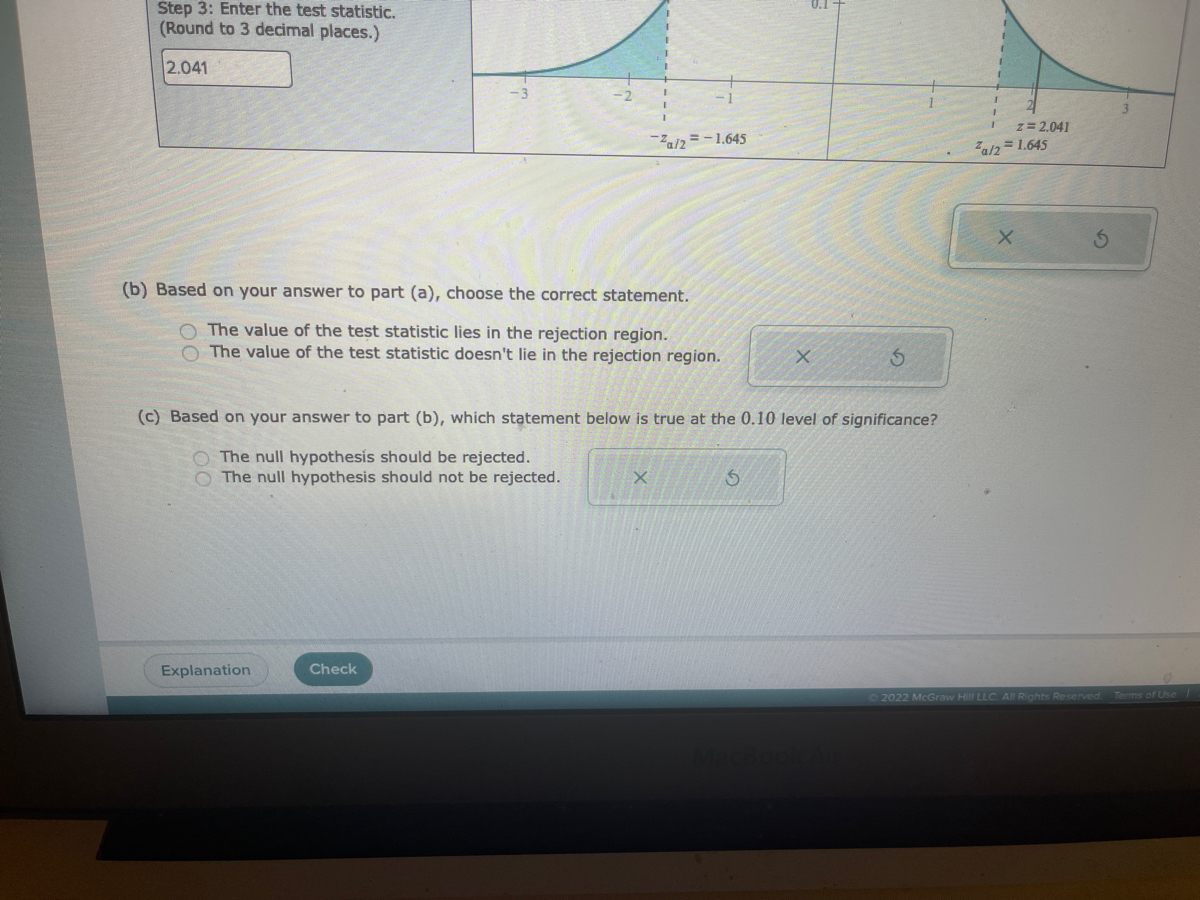

Transcribed Image Text:**Hypothesis Testing with Significance Level 0.10**
**Step 3: Enter the Test Statistic**
- Calculation: Round to 3 decimal places.
- Test Statistic Value: 2.041
**Visual Demonstration**
The image includes two bell curves on either side of the test statistic:
1. **Left Bell Curve:**
- The area under the curve to the left of \( z_{\alpha/2} = -1.645 \) is shaded, indicating the rejection region on the negative side.
2. **Right Bell Curve:**
- The area under the curve to the right of \( z = 2.041 \) is shaded, marking the rejection region on the positive side.
- The critical value is \( z_{\alpha/2} = 1.645 \).
**Decision Making**
**(b) Analyzing the Test Statistic:**
- Determine if the test statistic falls within the rejection region.
- Options:
- The value of the test statistic lies in the rejection region.
- The value of the test statistic doesn't lie in the rejection region.
- Response Options: Checkboxes next to each statement allow selection.
**(c) Conclusion at 0.10 Level of Significance:**
- Decide on the null hypothesis based on previous analysis.
- Options:
- The null hypothesis should be rejected.
- The null hypothesis should not be rejected.
- Response Options: Checkboxes next to each statement allow selection.
**Interactive Elements**
- Buttons for "Explanation" and "Check" findings.
This layout and questioning guide students through the concepts of hypothesis testing, focusing on critical thinking and accurate decision-making based on statistical evidence in a two-tailed test.
![Suppose there is a claim that a certain population has a mean, μ, that is different than 9. You want to test this claim. To do so, you collect a large random sample from the population and perform a hypothesis test at the 0.10 level of significance. To start this test, you write the null hypothesis \( H_0 \) and the alternative hypothesis \( H_1 \) as follows:
\[ H_0: \mu = 9 \]
\[ H_1: \mu \neq 9 \]
Suppose you also know the following information:
The critical values are -1.645 and 1.645 (rounded to 3 decimal places).
The value of the test statistic is 2.041 (rounded to 3 decimal places).
(a) Complete the steps below to show the rejection region(s) and the value of the test statistic for this test.
**Standard Normal Distribution**
- **Step 1:** Select one-tailed or two-tailed.
- One-tailed
- Two-tailed (selected)
- **Step 2:** Enter the critical value(s). (Round to 3 decimal places.)
- -1.645, 1.645
- **Step 3:** Enter the test statistic. (Round to 3 decimal places.)
- 2.041
**Graph Explanation:**
The graph represents a standard normal distribution. It is a bell-shaped curve centered around a mean of 0. The x-axis represents the z-scores, while the y-axis represents the probability density. Critical values of -1.645 and 1.645 are marked on the x-axis, creating two rejection regions in the tails of the distribution. The test statistic of 2.041 is plotted on the x-axis, falling into the rejection region on the right side.](https://content.bartleby.com/qna-images/question/b5da94fe-19e7-4c6f-a636-47d7a1fa1ee8/37a2c306-624b-41ea-a89b-50b5924c0fc2/glefgc9f_processed.jpeg)
Transcribed Image Text:Suppose there is a claim that a certain population has a mean, μ, that is different than 9. You want to test this claim. To do so, you collect a large random sample from the population and perform a hypothesis test at the 0.10 level of significance. To start this test, you write the null hypothesis \( H_0 \) and the alternative hypothesis \( H_1 \) as follows:
\[ H_0: \mu = 9 \]
\[ H_1: \mu \neq 9 \]
Suppose you also know the following information:
The critical values are -1.645 and 1.645 (rounded to 3 decimal places).
The value of the test statistic is 2.041 (rounded to 3 decimal places).
(a) Complete the steps below to show the rejection region(s) and the value of the test statistic for this test.
**Standard Normal Distribution**
- **Step 1:** Select one-tailed or two-tailed.
- One-tailed
- Two-tailed (selected)
- **Step 2:** Enter the critical value(s). (Round to 3 decimal places.)
- -1.645, 1.645
- **Step 3:** Enter the test statistic. (Round to 3 decimal places.)
- 2.041
**Graph Explanation:**
The graph represents a standard normal distribution. It is a bell-shaped curve centered around a mean of 0. The x-axis represents the z-scores, while the y-axis represents the probability density. Critical values of -1.645 and 1.645 are marked on the x-axis, creating two rejection regions in the tails of the distribution. The test statistic of 2.041 is plotted on the x-axis, falling into the rejection region on the right side.
Expert Solution
This question has been solved!
Explore an expertly crafted, step-by-step solution for a thorough understanding of key concepts.

This is a popular solution

Trending nowThis is a popular solution!

Step by stepSolved in 3 steps with 1 images

Knowledge Booster

Similar questions
- Does more education lower a person’s level of prejudice? The number of years of education and the score on a prejudice test for ten people is given in the following table. Higher scores on the test indicate more prejudice. Years of Education: 12, 15, 14, 13, 18, 10, 16, 12, 10, 4 Score of Prejudice Test: 1, 6, 2, 3, 2, 4, 1, 5, 5, 10 Conduct a hypothesis test to determine if there is a significant linear correlation between the two variables. If there is a significant linear correlation between the variables, determine the regression equation. There is a significant correlation between the variables and the regression equation is y' = 10.5 - 0.532x There is a significant correlation between the variables and the regression equation is y' = - 0.532 + 10.5x There is not a significant correlation between the variables, so the regression equation should not be determined. There is a significant correlation between the variables and the regression equation is y' = 16.509 - 1.054xarrow_forwardFind the test statistic Find the critical value What is the conclusionarrow_forwardIt's not for a test. The question is asking about a test:)arrow_forward
- Test the claim that the proportion of people who own cats is larger than 40% at the 0.1 significance level. Based on a sample of 500 people, 46% owned catsThe test statistic is: (to 2 decimals)The p-value is: (to 2 decimals)arrow_forwardfind p value and its meaning please A survey of 1000 adults from a certain region asked, "If purchasing a used car made certain upgrades or features more affordable, what would be your preferred luxury upgrade?" The results indicated that 58% of the females and 51% of the males answered window tinting. The sample sizes of males and females were not provided. Suppose that of 600 females, 348 reported window tinting as their preferred luxury upgrade of choice, while of 400 males, 204 reported window tinting as their preferred luxury upgrade of choice. Complete parts (a) through (d) below. a. Is there evidence of a difference between males and females in the proportion who said they prefer window tinting as a luxury upgrade at the 0.05 level of significance? State the null and alternative hypotheses, where π1 is the population proportion of females who said they prefer window tinting as a luxury upgrade and π2 is the population proportion of males who said…arrow_forwardThe table to the right contains observed values and expected values in parentheses for two categorical variables, X and Y, where variable X has three categories and variable Y has two categories. Use the table to complete parts (a) and (b) below. EQuestion Help X, X2 32 44 51 (35.39)(44.42)(47.19 19 20 17 (15.61)(19.58)(20.81) O B. H,: The Y category and X category have equal proportions. H,: The proportions are not equal. OC. Hn: The Y category andX category are dependent. H,: The Y category and X category are independent. OD. Ho: H -E, and Hy =E, H: H #E, or H, 7E, What is the P-value? P-value = (Round to three decimal places as needed.) Enter your answer in the answer box and then click Check Answer. portarrow_forward
- You want to study whether music affects people’s ability to learn. You have 10 college students study a list of words with soft classical music playing, then you test how many words they correctly remember. You have 15 different college students study a list of words with loud heavy metal playing, then you test how many words they correctly remember. You want to compare the learning/memory of the two different groups. What kind of hypothesis test should you do? One-Sample z-test One-Sample t-test Independent-Samples t-test Related-Samples t-testarrow_forwardDoes the type of instruction in a college statistics class (either lecture or self-paced) influence students’ performance, as measured by the number of quizzes successfully completed during the semester? Twelve students were recruited for the study. Students received the lecture instruction or a self-paced instruction. The total number of quizzes completed during teach type of instruction appear below.arrow_forwardTest the claim that the proportion of people who own cats is significantly different than 50% at the 0.02 significance level. Based on a sample of 100 people, 58% owned catsThe test statistic is: (to 2 decimals)The p-value is: (to 2 decimals)arrow_forward
arrow_back_ios
arrow_forward_ios
Recommended textbooks for you
- MATLAB: An Introduction with ApplicationsStatisticsISBN:9781119256830Author:Amos GilatPublisher:John Wiley & Sons Inc
 Probability and Statistics for Engineering and th...StatisticsISBN:9781305251809Author:Jay L. DevorePublisher:Cengage Learning
 Statistics for The Behavioral Sciences (MindTap C...StatisticsISBN:9781305504912Author:Frederick J Gravetter, Larry B. WallnauPublisher:Cengage Learning
  Elementary Statistics: Picturing the World (7th E...StatisticsISBN:9780134683416Author:Ron Larson, Betsy FarberPublisher:PEARSON
 The Basic Practice of StatisticsStatisticsISBN:9781319042578Author:David S. Moore, William I. Notz, Michael A. FlignerPublisher:W. H. Freeman
 Introduction to the Practice of StatisticsStatisticsISBN:9781319013387Author:David S. Moore, George P. McCabe, Bruce A. CraigPublisher:W. H. Freeman
MATLAB: An Introduction with Applications
Statistics
ISBN:9781119256830
Author:Amos Gilat
Publisher:John Wiley & Sons Inc
Probability and Statistics for Engineering and th...
Statistics
ISBN:9781305251809
Author:Jay L. Devore
Publisher:Cengage Learning
Statistics for The Behavioral Sciences (MindTap C...
Statistics
ISBN:9781305504912
Author:Frederick J Gravetter, Larry B. Wallnau
Publisher:Cengage Learning
Elementary Statistics: Picturing the World (7th E...
Statistics
ISBN:9780134683416
Author:Ron Larson, Betsy Farber
Publisher:PEARSON
The Basic Practice of Statistics
Statistics
ISBN:9781319042578
Author:David S. Moore, William I. Notz, Michael A. Fligner
Publisher:W. H. Freeman
Introduction to the Practice of Statistics
Statistics
ISBN:9781319013387
Author:David S. Moore, George P. McCabe, Bruce A. Craig
Publisher:W. H. Freeman