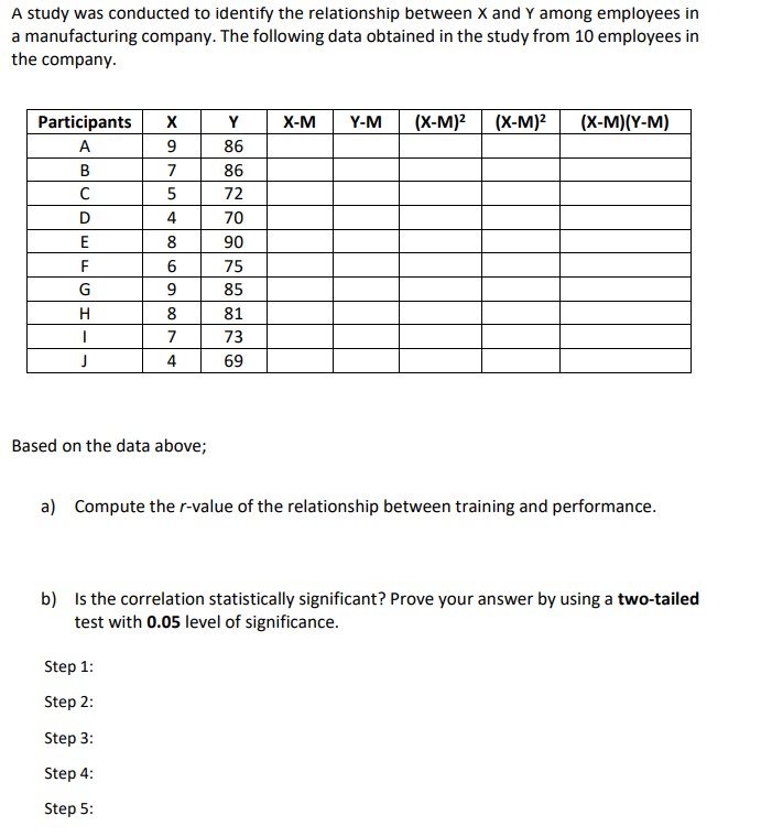
A study was conducted to identify the relationship between X and Y among employees in a manufacturing company. The following data obtained in the study from 10 employees in the company. Participants X Y X-M Y-M (X-M)² (X-M)² (X-M)(Y-M) A 9 86 B 7 86 C 5 72 D 4 70 E 8 90 F 6 75 G 9 85 H 8 81 I 7 73 J 4 69 Based on the data above; a) Compute the r-value of the relationship between training and performance. b) Is the correlation statistically significant? Prove your answer by using a two-tailed test with 0.05 level of significance. Step 1: Step 2: Step 3: Step 4: Step 5:

The authors of a paper compared two different methods for measuring body fat percentage. One method uses ultrasound, and the other method uses X-ray technology. Body fat percentages using each of these methods for 16 athletes (a subset of the data given in a graph that appeared in the paper) are given in the accompanying table. You can assume that the 16 athletes who participated in this study are representative of the population of athletes. Athlete X-ray Ultrasound 1 5.00 4.25 2 12.00 8.75 3 9.25 9.00 4 12.00 11.75 5 17.25 17.00 6 29.50 27.50 7 5.50 6.50 8 6.00 6.75 9 8.00 8.75 10 9.50 10.50 11 9.25 9.50 12 11.00 12.00 13 12.00 12.25 14 14.00 15.50 15 17.00 18.00 16 18.00 18.25   Use these data to estimate the difference in mean body fat percentage measurement for the two methods. Use a confidence level of 95%. (Use ?d = ?X-ray − ?ultrasound. Round your answers to three decimal places.)     ,     % Interpret the interval in…

An article gave the following data on y = number of employees in fiscal year 2007–2008 and x = total size of parks (in acres) for the 20 state park districts in a state. Number of Employees, y Total Park Size, x 95 39,334 95 324 102 17,315 69 8,244 67 620,231 77 43,501 81 8,625 116 31,572 51 14,276 36 21,095 96 103,289 71 130,023 76 16,068 112 3,286 43 24,089 87 6,309 131 14,502 138 62,595 80 23,666 52 35,832 (a) Construct a scatterplot of the data. A scatterplot has 20 points. The horizontal axis is labeled "x" and ranges from 0 to 700,000.The vertical axis is labeled "y" and ranges from 0 to 150.The points are scattered mostly between approximately 0 and 150,000 on the horizontal axis and between approximately 35 and 140 on the vertical axis. One point is located at approximately (625,000, 65). A scatterplot has 20 points. The horizontal axis is labeled "x" and ranges from 0 to 700,000.The vertical axis is labeled "y" and ranges from 0 to 150.The points are scattered mostly between…

A psychologist at a private mental health facility was asked to determine whether there was a clear difference in the length of stay for patients with different categories of diagnosis. Looking at the last seven patients in each of the three major categories, the results (in terms of weeks of stay) were as follows. Using the data below, test whether the length of stay for patients vary based on category of diagnosis.  Diagnosis Category  Affective Disorders  Cognitive Disorders  Drug-related Conditions  7 12 8 6 8 10 5 9 12 6 11 10 9 11 9 5 10 11 6 9 12 The above scenario requires a one-way Anova, with a bar graph. Question - I need to write an explanation for the output given. I am to include a statistical notation and explanation as to whether the results are significant or not significant.  Examples of Explanation: Non-significant:A One-Way ANOVA was conducted to examine whether a preceding situation (watching a…