
ENGR.ECONOMIC ANALYSIS
14th Edition
ISBN: 9780190931919
Author: NEWNAN
Publisher: Oxford University Press
expand_more
expand_more
format_list_bulleted
Question
- A multiple regression model, K = a + bX + cY + dZ, is estimated regression software, which produces the following output:
a. Are the estimates of a, b, c, and d statistically significant at the 1 percent significance level?
b. How much of the total variation is explained by this regression equation?
c. Is the overall regression equation statistically significant at the 1 percent level of significance?
d. If X equals 50, Y equals 200, and Z equals 45, what value do you predict K will take?
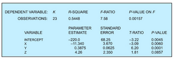
Transcribed Image Text:DEPENDENT VARIABLE: K
23
OBSERVATIONS:
VARIABLE
INTERCEPT
X
<> N
Y
R-SQUARE
0.5448
PARAMETER
ESTIMATE
-220.0
-11.340
0.3875
4.26
F-RATIO
7.58
STANDARD
ERROR
68.25
3.670
0.0625
2.350
P-VALUE ON F
0.00157
T-RATIO
-3.22
-3.09
6.20
1.81
P-VALUE
0.0045
0.0060
0.0001
0.0857
Expert Solution
This question has been solved!
Explore an expertly crafted, step-by-step solution for a thorough understanding of key concepts.
This is a popular solution
Trending nowThis is a popular solution!
Step by stepSolved in 3 steps with 5 images

Knowledge Booster
Learn more about
Need a deep-dive on the concept behind this application? Look no further. Learn more about this topic, economics and related others by exploring similar questions and additional content below.Similar questions
- Suppose you have run four regression models: A, B, C, and D. You are going to make a decision on which one to use just based on the adjusted r² value. Here are the adjusted r² values for each model: A: 0.71 B: 0.57 C: 0.65 D: 0.76 Which regression model would you choose based on the adjusted r²? OD since it has the highest adjusted r² value B since it has the lowest adjusted r² OC since it has an adjusted r² between the adjusted r² of regressions B and D. Either B or C since they have the lowest adjusted r²arrow_forwardConsider the simple two-variable linear regression model y₁ = Bo + Bixi + e¡ with unknown parameters Boand B₁ and s, is the unobserved random error term. The corresponding OLS regression equation for the above model is: 9 = Bo + B₁x + ₁, where hats indicated estimates of the coefficients and residuals. Given this information, what is the OLS criterion? a. min Σ. ΣΤΟ -1) b. min E *Σ(βο + β1x.) c. min E ê-E-Bo + B₂x₁) d. min ΣτêΣΟ - β - β,x) e. min Σ€ΣΟ - β) a b Oc Odarrow_forwardInstructions: Submit a well-formatted Word, pdf, or similar file in Canvas with your R scripts, regression output, and answers to the questions below. This lab exercise asks you to evaluate the housing market. The data set housingprices40.csv contains all sales of single-family homes in Davis, CA in May 2018 (n = 40). Assume that these homes are a random sample. The dependent variable in the regression model is the natural logarithm of the actual price of each house sold. The regression specification is: In(price;) = B2 + B2 In(estimate;) + B3bdrms; + B4bathrms; +B; In(sqrft;) + B6 In(lotsize}) + Brage; + Bapooli+Bocentrali + & where price is the house selling price, estimate is the estimated housing value from April 2018 from a prominent online site that values homes, bdrms is the number of bedrooms, bathrms is the number of bathrooms, sqrft is the interior square footage, lotsize is size of the lot (in feet), age is the age of the house in years, pool is a binary variable set to…arrow_forward
- Imagine you are an economist working for the Government of Econville. You are tasked with developing a model to predict the GDP of the country based on various factors such as interest rates, inflation, unemployment rate, and population growth. You collect quarterly data for the past 20 years and start building your model. After running your initial regression, you notice some peculiar patterns in the residuals: (1) residuals do not have identical variances across different levels of the independent variables; (2) two or more independent variables in a regression model are highly correlated with each other; (3) the correlation of a variable with its own past values. You suspect that your model might be suffering from 3 potential issues in the regression analysis that can affect reliability and validity. List 2 factors in your model that might be causing the Multicollinearity and give a reasonarrow_forwardThe data for this question is given in the file 1.Q1.xlsx(see image) and it refers to data for some cities X1 = total overall reported crime rate per 1 million residents X3 = annual police funding in $/resident X7 = % of people 25 years+ with at least 4 years of college (a) Estimate a regression with X1 as the dependent variable and X3 and X7 as the independent variables. (b) Will additional education help to reduce total overall crime (lead to a statistically significant reduction in crime)? Please explain. (c) Will an increase in funding for the police departments help reduce total overall crime (lead to a statistically significant reduction in total overall crime)? Please explain. (d) If you were asked to recommend a policy to reduce crime, then, based only on the above regression results, would you choose to invest in education (local schools) or in additional funding for the police? Please explain.arrow_forwardThis exercise refers to the drunk driving panel data regression summarized below. Regression Analysis of the Effect of Drunk Driving Laws on Traffic Deaths Dependent variable: traffic fatility rate (deaths per 10,000). Regressor Beer tax Drinking age 18 Drinking age 19 Drinking age 20 Drinking age Mandatory jail or community service? Average vehicle miles per driver Unemployment rate Real income per capita (logarithm) Years State Effects? Time effects? (1) 0.41* (0.056) 1982-88 no no (2) (3) (4) -0.62** -0.76*** -0.42 (0.39) (0.33) (0.38) 0.023 (0.078) -0.014 (0.084) -0.023 -0.075 (0.053) (0.064) 0.034 -0.109*** (0.058) (0.058) no yes yes no yes Clustered standard errors? yes yes F-Statistics and p-Values Testing Exclusion of Groups of Variables Time effects=0 (5) -0.76** (0.36) 0.041 0.083 (0.111) (0.115) 0.006 0.015 (0.005) (0.011) -0.068* (0.016) 1.66* (0.66) 1982-88 1982-88 1982-88 1982-88 yes yes yes yes yes yes (6) -0.46 (0.39) -0.004 (0.022) 0.043 (0.101) 0.007 (0.005) -0.064*…arrow_forward
- The data below represent commute times (in minutes) and scores on a well-being survey. Complete parts (a) through (d) below. Commute Time (minutes), x Well-Being Index Score, y 5 72 105 20 25 35 60 69.2 68.0 67.5 67.1 65.9 66.0 63.8 (a) Find the least-squares regression line treating the commute time, x, as the explanatory variable and the index score, y, as the response variable. ŷ=x+ (Round to three decimal places as needed.) (b) Interpret the slope and y-intercept, if appropriate. First interpret the slope. Select the correct choice below and, if necessary, fill in the answer box to complete your choice. OA. For every unit increase in commute time, the index score falls by (Round to three decimal places as needed.) OB. For every unit increase in index score, the commute time falls by (Round to three decimal places as needed.) 1 D. For an index score of zero, the commute time is predicted to be (Round to three decimal places as needed.) on average. on average. OC. For a commute time…arrow_forwardIn a regression problem with one output variable and one input variable, we set up two cutpoints z1 and z2 for the input variable and we fit a step function regression model based on these two cutpoints of the input variable. If you write the regression problem in matrix form y = X%*%β + ε, how many rows would the vector β have?arrow_forwardGiven the estimated multiple regression equation ŷ = 6 + 5x1 + 4x2 + 7x3 + 8x4 what is the predicted value of Y in each case? a. x1 = 10, x2 = 23, x3 = 9, and x4 = 12 b. x1 = 23, x2 = 18, x3 = 10, and x4 = 11 c. x1 = 10, x2 = 23, x3 = 9, and x4 = 12 d. x1 = -10, x2 = 13, x3 = -8, and x4 = -16arrow_forward
- Hello, please help me to solve the question (c) and (d) below.Consider this regression model (1) : Yt = β0 + β1 Ut + β2 Vt + β3 Wt + β4 Xt + εt ; where t= 1, ..., 75.We use OLS to estimate the parameters, producing the following model:Ŷt = 1.115 + 0.790 Ut − 0.327 Vt + 0.763 Wt + 0.456 Xt (0.405) (0.178) (0.088) (0.274) (0.017) Given that:R2 = 0.941; Durbin Watson stat DW = 1.907; RSS = 0.0757.(To answer the question, use the 5% level of significance, state clearly H0 and H1 that are tested, the test statistics that are used, and interpret the decisions.) (a) Describe the concepts of unbiasedness and efficiency. State the conditions required of regression (1) in order that the OLS estimators of the model parameters possess these properties. (b) Perform the following tests on the parameters of regression (1): (i) test whether the parameters β1, β2, β3 and β4 are individually statistically significant; (ii) test the overall significance of the regression model;…arrow_forwardplease answer in text form and in proper format answer with must explanation , calculation for each part and steps clearlyarrow_forwardImagine you are an economist working for the Government of Econville. You are tasked with developing a model to predict the GDP of the country based on various factors such as interest rates, inflation, unemployment rate, and population growth. You collect quarterly data for the past 20 years and start building your model. After running your initial regression, you notice some peculiar patterns in the residuals: (1) residuals do not have identical variances across different levels of the independent variables; (2) two or more independent variables in a regression model are highly correlated with each other; (3) the correlation of a variable with its own past values. You suspect that your model might be suffering from 3 potential issues in the regression analysis that can affect reliability and validity. what are the implications of Heteroscedasticity if this potential issue in your model?arrow_forward
arrow_back_ios
SEE MORE QUESTIONS
arrow_forward_ios
Recommended textbooks for you

 Principles of Economics (12th Edition)EconomicsISBN:9780134078779Author:Karl E. Case, Ray C. Fair, Sharon E. OsterPublisher:PEARSON
 Engineering Economy (17th Edition)EconomicsISBN:9780134870069Author:William G. Sullivan, Elin M. Wicks, C. Patrick KoellingPublisher:PEARSON
 Principles of Economics (MindTap Course List)EconomicsISBN:9781305585126Author:N. Gregory MankiwPublisher:Cengage Learning
 Managerial Economics: A Problem Solving ApproachEconomicsISBN:9781337106665Author:Luke M. Froeb, Brian T. McCann, Michael R. Ward, Mike ShorPublisher:Cengage Learning
 Managerial Economics & Business Strategy (Mcgraw-...EconomicsISBN:9781259290619Author:Michael Baye, Jeff PrincePublisher:McGraw-Hill Education


Principles of Economics (12th Edition)
Economics
ISBN:9780134078779
Author:Karl E. Case, Ray C. Fair, Sharon E. Oster
Publisher:PEARSON

Engineering Economy (17th Edition)
Economics
ISBN:9780134870069
Author:William G. Sullivan, Elin M. Wicks, C. Patrick Koelling
Publisher:PEARSON

Principles of Economics (MindTap Course List)
Economics
ISBN:9781305585126
Author:N. Gregory Mankiw
Publisher:Cengage Learning

Managerial Economics: A Problem Solving Approach
Economics
ISBN:9781337106665
Author:Luke M. Froeb, Brian T. McCann, Michael R. Ward, Mike Shor
Publisher:Cengage Learning

Managerial Economics & Business Strategy (Mcgraw-...
Economics
ISBN:9781259290619
Author:Michael Baye, Jeff Prince
Publisher:McGraw-Hill Education