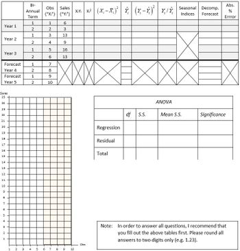
Questions 1-30 refer to the following scenario: A company reports bi-annual (twice a year) sales data. The sales data for the last three years is shown in below Table.
The intercept (a) of the regressions line (DV: Sales, IV: Obs) is equal to
|
A
|
2 |
|
B
|
4 |
|
C
|
3 |
|
D
|
1 |
The slope (b) of the regressions line (DV: Sales, IV: Obs) is equal to
| a |
4 |
| b |
2 |
| c |
3 |
| d |
1 |
The standard error of the regression is
| a |
5.34 |
| b |
3.54 |
| c |
4.35 |
| d |
2.51 |
The standard error of the intercept is
| a |
1.30 |
| b |
2.30 |
| c |
0.30 |
| d |
3.30 |
You want to test the hypothesis that the intercept is statistically significantly different from zero. To do so, you use the attached t-table. Your alpha (the risk you accept to make a Type I error) is a=0.1. How many degrees of freedom do you have?
| a |
n |
| b |
n-2 |
| c |
4 |
| d |
both b. and c. are correct |
You want to test the hypothesis that the intercept is statistically significantly different from zero. To do so, you use the attached t-table. Your alpha (the risk you accept to make a Type I error) is a=0.1. What is your t-statistic to conduct the hypothesis test?
| a |
t=0.71 |
| b |
t=0.81 |
| c |
t=0.91 |
| d |
t=1.01 |
The standard error of the slope is
| a |
0.95 |
| b |
1.15 |
| c |
1.05 |
| d |
0.85 |
You want to test the hypothesis that the slope coefficient is statistically significantly different from zero. To do so, you use the attached t-table. Your alpha (the risk you accept to make a Type I error) is a=0.1. What is your t-statistic to conduct the hypothesis test?
| a |
4.35 |
| b |
3.35 |
| c |
2.35 |
| d |
1.35 |
Which statement is true? Given your alpha of a=0.1, you
| a |
Reject the null for the intercept, and fail to reject the null for the slope |
| b |
Reject the null for the slope, and fail to reject the null for the intercept |
| c |
Fail to reject the null for both the intercept and the slope |
| d |
Reject the null for both the intercept and the slope |
The explained sum of squares of the regression is ESS =
| a |
20 |
| b |
120 |
| c |
70 |
| d |
50 |
Trending nowThis is a popular solution!
Step by stepSolved in 5 steps with 1 images

- Please answerarrow_forwardPlease provide the correct answer along with the calculation. Do not use ChatGPT, otherwise I will give a downvote.arrow_forwardYou estimated a regression with the following output. Source | SS df MS Number of obs = 411 -------------+---------------------------------- F(1, 409) = 4098.54 Model | 22574040.7 1 22574040.7 Prob > F = 0.0000 Residual | 2252702.97 409 5507.83122 R-squared = 0.9093 -------------+---------------------------------- Adj R-squared = 0.9090 Total | 24826743.7 410 60553.0334 Root MSE = 74.215 ------------------------------------------------------------------------------ Y | Coef. Std. Err. t P>|t| [95% Conf. Interval] -------------+---------------------------------------------------------------- X | 6.727341 .1050822 64.02 0.000 6.520772 6.933909 _cons | -.7552724 9.26027 -0.08 0.935 -18.95894 17.44839…arrow_forward
- An analyst working for your firm provided an estimated log-linear demand function based on the natural logarithm of the quantity sold, price, and the average income of consumers. Results are summarized in the following table: SUMMARY OUTPUT Regression Statistics Multiple R R Square Adjusted R Square Standard Error Observations ANOVA Regression Residual Total Intercept LN Price LN Income df 0.968 0.937 0.933 0.003 30 SS MS F 2 0.003637484 0.001818742 202.48598 0.000242516 8.98206E-06 27 29 0.00388 Coefficients Standard Error 0.57 0.00 0.13 0.51 -0.08 0.15 t Stat 0.90 -19.50 1.13 P-value 0.37 0.00 0.27 Significance F 5.55598E-17 Lower 95% -0.65 -0.09 -0.12 How would a 4 percent increase in income impact the demand for your product? Demand would increase by 60 percent. Demand would increase by 0.6 percent. Demand would decrease by 60 percent. Demand would decrease by 0.6 percent. Upper 95% 1.68 -0.07 0.41arrow_forwardPlease provide me with the correct answer, along with the calculations, and do not use any AI toolsarrow_forwardQUESTION 10 Answer questions 10 to 16 based on the regression outputs given in Table 1& 2. Table 1 DATA4-1: Data on single family homes in University City community of San Diego, in 1990. price - sale price in thousands of dollars (Range 199. 9 505) sqft - square feet of living area (Range 1065 - 3000) Table 2 Model 1: OLS, using observations 1-14 Dependent variable: price coefficient std. error t-ratio p-value 52. 3509 0.138750 37. 2855 0.0187329 0. 1857 8. 20e-06 *** const sqft 7. 407 Me dependent var Sun squared resid R-squared F(1, 12) Log-likelihood Schwarz criterion 317. 4929 18273. 57 0. 820522 54. 86051 -70. 08421 145. 4465 Hannan-Quinn S.D. dependent var S.E. of regression Adjusted R-squared P-value (F) Akaike criterion 88. 49816 39. 02304 0. 805565 8. 20e-06 144. 1684 144. 0501 There are observations included in this dataset. It is a. data. O 12; cross-sectional 13; time-series data 14; cross-sectional In this regression model, sale price of a single-family house is the. the…arrow_forward
- The data for this question is given in the file 1.Q1.xlsx(see image) and it refers to data for some cities X1 = total overall reported crime rate per 1 million residents X3 = annual police funding in $/resident X7 = % of people 25 years+ with at least 4 years of college (a) Estimate a regression with X1 as the dependent variable and X3 and X7 as the independent variables. (b) Will additional education help to reduce total overall crime (lead to a statistically significant reduction in crime)? Please explain. (c) Will an increase in funding for the police departments help reduce total overall crime (lead to a statistically significant reduction in total overall crime)? Please explain. (d) If you were asked to recommend a policy to reduce crime, then, based only on the above regression results, would you choose to invest in education (local schools) or in additional funding for the police? Please explain.arrow_forwardThe dependent variable in the regression in our cost driver analysis is which of the following? Company sales Total overhead cost for the entire period of time Total overhead cost per montharrow_forward18 Calculate the least square regression líne equation with the given X and Y values. Consider the values: X Y 60 3.1 61 3.6 62 3.8 63 4 65 4.1 To Find, Least Square Regression Line EquationY = a+ b Xarrow_forward
- Consider the following regression model and corresponding output for a dataset with n = 104 observations: y=ß₁+ß2x2+ß³¸*¸+4 3 4x4+u Variable β Std. Error t P>|t| X2 -0.012 0.006 -2.289 0.022 X3 0.596 0.014 41.139 0.000 X4 0.52 1.06 Constant 8.860 1.766 5.017 0.000 What is the marginal effect of x4 on y? (approximate at least to 3 decimal places)arrow_forwardThe following question refers to this regression equation (standard errors for each of the estimated coefficients are in parenthesis). Q=8,400-8" P+5" A+ 4** Px +0.05**1, (1,732) (2.29) (1.36) (1.75) (0.15) Q = Quantity demanded P = Price 1,100 Advertising expenditures, in thousands = 20 P = price of competitor's good = 600/= average monthly income 10,000 What is the advertising elasticity of demand? Round your answer to two decimal places. Your Answer: The t-statistic is computed by dividing the regression coefficient by the standard error of the coefficient. dividing the regression coefficient by the standard error of the estimate. dividing the standard error of the coefficient by the regression coefficient. dividing the R2 by the F-statistic. none of the specified answers are correct.arrow_forwardYou estimated a regression with the following output. Source | SS df MS Number of obs = 268 -------------+---------------------------------- F(1, 266) = 23.48 Model | 668419.175 1 668419.175 Prob > F = 0.0000 Residual | 7572666.51 266 28468.6711 R-squared = 0.0811 -------------+---------------------------------- Adj R-squared = 0.0777 Total | 8241085.68 267 30865.4895 Root MSE = 168.73 ------------------------------------------------------------------------------ Y | Coef. Std. Err. t P>|t| [95% Conf. Interval] -------------+---------------------------------------------------------------- X | 1.014128 .2092916 4.85 0.000 .6020489 1.426207 _cons | 9.173163 21.13463 0.43 0.665 -32.43929 50.78561…arrow_forward

 Principles of Economics (12th Edition)EconomicsISBN:9780134078779Author:Karl E. Case, Ray C. Fair, Sharon E. OsterPublisher:PEARSON
 Engineering Economy (17th Edition)EconomicsISBN:9780134870069Author:William G. Sullivan, Elin M. Wicks, C. Patrick KoellingPublisher:PEARSON
 Principles of Economics (MindTap Course List)EconomicsISBN:9781305585126Author:N. Gregory MankiwPublisher:Cengage Learning
 Managerial Economics: A Problem Solving ApproachEconomicsISBN:9781337106665Author:Luke M. Froeb, Brian T. McCann, Michael R. Ward, Mike ShorPublisher:Cengage Learning
 Managerial Economics & Business Strategy (Mcgraw-...EconomicsISBN:9781259290619Author:Michael Baye, Jeff PrincePublisher:McGraw-Hill Education
