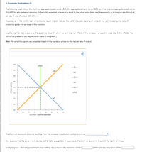
9. Economic fluctuations II The following graph shows the short-run aggregate-supply curve (AS), the aggregate-demand curve (AD), and the long-run aggregate-supply curve (LRAS) for a hypothetical economy. Initially, the expected price level is equal to the actual price level, and the economy is in long-run equilibrium at its natural rate of output, $80 billion. Suppose war in the world's main oil-producing region sharply reduces the world oil supply, causing oil prices to rise and increasing the costs of producing goods and services in this economy. Use the graph to help you answer the questions about the short-run and long-run effects of the increase in production costs that follow. (Note: You will not be graded on any adjustments made to the graph.) Hint: For simplicity, ignore any possible impact of the higher oil prices on the natural rate of output. 100 LRÅS 95 AS AD 90 85 AS 80 LRAS 75 70 AD 65 60 60 65 70 75 80 85 90 95 100 OUTPUT (Billions of dollars) The short-run economic outcome resulting from the increase in production costs is known as Now suppose that the government decides not to take any action in response to the short-run economic impact of the higher oil prices. In the long-run, when the government does nothing, the output in the economy will be s billion and the price level will be PRICE LEVEL

Pessimism (suggestion: draw the AS-AD diagram to help your analysis and start with the long-run and short-run equilibrium, i.e. the intersection of LRAS, SRAS and AD curves) Suppose the economy is in long-run equilibrium. Then because of corporate scandal, international tensions, and loss of confidence in policymakers, people become pessimistic regarding the future and retain that level of pessimism for some time. Refer to Pessimism. In the short run what happens to the price level and real GDP? O 1) Both the price level and real GDP rise. 2) Both the price level and real GDP fall. 3) The price level rises and real GDP falls. 4) The price level falls and real GDP rises.

2. The theory of liquidity preference and the downward-slopingaggregate demand curve Suppose the money market for some hypothetical economy is given by the following graph, which plots the money demand and money supply curves. Assume the central bank in this economy (the Fed) fixes the quantity of money supplied. Suppose the price level increases from 90 to 105. Shift the appropriate curve on the graph to show the impact of an increase in the overall price level on the market for money. INTEREST RATE (Percent) 18 15 12 8 3 0 0 20 Money Supply Money Demand 40 60 80 MONEY (Billions of dollars) 100 120 Money Demand Money Supply Following the price level increase, the quantity of money demanded at the initial interest rate of 9% will be supplied by the Fed at this interest rate. As a result, individuals will attempt to bonds and other interest-bearing assets, and bond issuers will realize that they restored in the money market at an interest rate of % than the quantity of money their money…

Following an increase in consumer confidence, the US economy is experiencing a significant increase in aggregate spending. Using a correctly labeled aggregate demand and aggregate supply diagram, show how the change in aggregate spending will affect each of the following in the short run -Output -The price level

Identify how each of the following changes will affect Aggregate Demand An increase in consumers disposable income A decrease in Investment spending due to pessimistic forecasts concerning the future A global pandemic resulting in business closures and an increase in the unemployment level The federal government increases spending on roads, bridges, and school repairs The federal government reduces the federal income tax resulting in an increase in household disposable income

Interpret the change you drew on the previous graph by filling in the blanks in the following paragraph: The lower-than-expected price level causes firms to earn more profit than they expected on each unit of output they produce, and, therefore, they decrease their production level. At the same time, the real value of wages and other resource prices are lower than workers and firms expected when they signed long-term contracts. As a result, the economy as a whole produces at a level below the unemployment rate is lower than its natural rate. its potential output, and Now, suppose prices remain lower than expected. As a result, in the next round of labor negotiations, unions accept lower wages for their members. The following graph shows the potential output for this economy as well as the same initial short-run aggregate supply curve as in the first graph. Shift one or both of these lines to illustrate how the economy adjusts to a new long-run equilibrium. PRICE LEVEL 180 SRAS 150…

The following events have occurred at times in the history of the United States: 1. The world economy goes into an expansion. 2. U.S. businesses expect future profits to rise. 3. The government increases its expenditure on goods and services in a time of war or increased international tension. Explain the combined effects of these events on U.S. real GDP and the price level, starting from a position of long-run equilibrium. The graph shows an economy in long-run equilibrium. The world economy goes into an expansion, U.S. businesses expect future profits to rise, and the government increases its expenditure on goods and services in a time of war or increased international tension. Draw one new curve that shows the combined effect of the three events. Label it. Draw a point at the new short-run macroeconomic equilibrium. 140- 130- Price level (GDP deflator, 2012=100) 120- 110- 100- 90- 80- 18.0 LAS SAS AD G 19.0 20.0 21.0 Real GDP (trillions of 2012 dollars) Denonh: the ohiarte conciliad…

Price Level a b c AS AD AD₁ Real GDP Refer to the figure above. If the aggregate supply curve shifted from ASo to AS₁, we could say that: aggregate supply has increased, and the equilibrium price level has risen to Og aggregate supply has decreased, equilibrium real output has increased, and the equilibrium price level has decreased aggregate supply has decreased, equilibrium real output has decreased, and the equilibrium price level has increased aggregate supply has increased, equilibrium real output has decreased, and the equilibrium price level has increased an increase in the amount of real output supplied has occurred

Answer both questions that need to be answered and the second question has a graph that’s needs to be answered as well.

Consider a fictional economy that is operating at its long-run equilibrium. The following graph shows the aggregate demand (AD) curve and short-run aggregate supply (AS) curve for the economy. The long-run aggregate supply curve is represented by a vertical line at the potential GDP level of $6 trillion. The economy is initially producing at potential GDP. Suppose that fiscal authorities decide to decrease marginal tax rates. Assume that this change in marginal tax rates is perceived as a long-term change. Shift the appropriate curves to illustrate the supply-side view of the fiscal policy effect on output and the price level. Note: Select and drag one or both of the curves to the desired position. Curves will snap into position, so if you try to move a curve and it snaps back to its original position, just drag it a little farther. 120 Potential GDP AS 100 PRICE LEVEL 60 80 60 40 40 20 20 0 0 2 4 6 8 AD 10 12 QUANTITY OF OUTPUT (Trillions of dollars) AD 1 AS Potential GDP True or…