
Whether there was a statistically significant difference in the average speeds, the mean speed, standard deviation, 85th percentile speed and percentage of traffic exceeding the posted speed limit of 30 mi/h.
Answer to Problem 9P
Significant reduction
Explanation of Solution
Given:
Significance level of
Formula used:
S is standard deviation
N is number of observations
Spis square root of the pooled variance
S1 and S2 are standard deviations of the populations
T is the test static
Calculation:
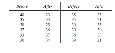
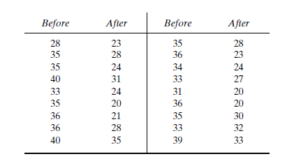
Before an increase in speed enforcement activities:
The speed ranges from 28 to 40 mi/hgiving a speed range of 12. For five classes, the range per class is 2.4mi/h. A frequency distribution table can then be prepared, as shown below, in which the speed classes are listed in column 1 and the mid-values are in column 2. The number of observationsfor each class is listed in column 3, the cumulative percentages of all observations arelisted in column 6.
| 1 | 2 | 3 | 4 | 5 | 6 | 7 |
| Speed class (mi/h) | Class mid-value | Class frequency, | | Percentage of class frequency | Cumulative percentage of class frequency | |
| 28-30 | 29 | 4 | 116 | 13 | 13 | 139.24 |
| 31-33 | 32 | 5 | 160 | 17 | 30 | 42.05 |
| 34-36 | 35 | 12 | 420 | 40 | 70 | 0.12 |
| 37-39 | 38 | 6 | 228 | 20 | 90 | 57.66 |
| 40-42 | 41 | 3 | 123 | 10 | 100 | 111.63 |
| Total | 30 | 1047 | 350.7 |
Determine the arithmetic mean speed:
Determine the standard deviation:
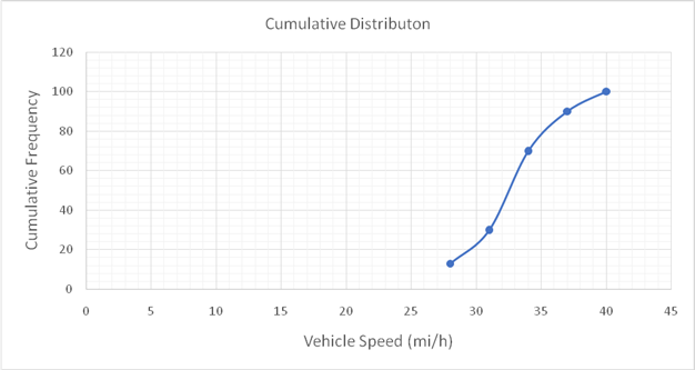
The 85th-percentile speed is obtained from the cumulative frequency distribution curve as 36 mi/h.
The percentage of traffic exceeding the posted speed limit of 30 mi/h is 76 %.
Below given figure shows the cumulative frequency distribution curve for the data given. In this case, the cumulative percentages in column 6 of the above Table are plotted against the upper limit of each corresponding speed class. This curve, therefore, gives the percentage of vehicles that are traveling at or below a given speed.
After an increase in speed enforcement activities:
The speed ranges from 20 to 37 mi/h giving a speed range of 17. For six classes, the range per class is 2.83 mi/h. A frequency distribution table can then be prepared, as shown below in which the speed classes are listed in column 1 and the mid-values are in column 2. The number of observations for each class is listed in column 3, the cumulative percentages of all observations are listed in column 6.
| 1 | 2 | 3 | 4 | 5 | 6 | 7 |
| Speed class (mi/h) | Class mid-value | Class frequency, | | Percentage of class frequency | Cumulative percentage of class frequency | |
| 20-22 | 21 | 6 | 126 | 20 | 20 | 253.5 |
| 23-25 | 24 | 8 | 192 | 27 | 47 | 98 |
| 26-28 | 27 | 4 | 108 | 13 | 60 | 1 |
| 29-31 | 30 | 3 | 90 | 10 | 70 | 18.75 |
| 32-34 | 33 | 5 | 165 | 17 | 87 | 151.25 |
| 35-37 | 36 | 4 | 144 | 13 | 100 | 289 |
| Total | 30 | 825 | 811.5 |
Determine the arithmetic mean speed:
Determine the standard deviation:
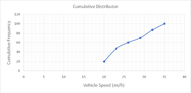
Below given figure shows the cumulative frequency distribution curve for the data given. In this case, the cumulative percentages in column 6 of the above Table are plotted against the upper limit of each corresponding speed class. This curve, therefore, gives the percentage of vehicles that are traveling at or below a given speed.
The 85th-percentile speed is obtained from the cumulative frequency distribution curve as 31.5 mi/h.
The percentage of traffic exceeding the posted speed limit of 30 mi/h is 24 %.
Determine square root of the pooled variance:
Compute test static T:
Determine whether
From Appendix A, theoretical
Since
Conclusion:
The increase in speed enforcement activities has resulted in a significant reduction in the mean speed on the street at a significance level of 0.05. The mean speeds before and after increase in speed enforcement activities are 35.1 and 27.47 mi/h respectively. The standard deviations are 3.5 and 5.3 mi/h respectively. The 85th percentile speeds are 36 mi/h and 31.5 mi/h and percentages of traffic exceeding the posted speed limit of 30 mi/h are 76 % and 24 %.
Want to see more full solutions like this?
Chapter 4 Solutions
Traffic and Highway Engineering

- 4) A spot speed study conducted on Sacramento State campus reported an average speed of 28.51 mph with 5.75 mph as standard deviation. Assuming that speeds have a normal distribution, what is the probability of speeding on Sacramento State campus (speed limit = 25 mph)?arrow_forwardA before-and-after speed study was conducted to determine the effectiveness of a series of rumble strips installed approaching a toll plaza to reduce approach speeds to 40 mi/h. The table below shows summarizes the results of the study. Item Average Speed Standard Deviation Sample Size O True Before Study 43.5 mi/h Ⓒ False 4.8 mi/h 120 After Study 40.8 mi/h 5.3 mi/h Answer the following True/False question after performing statistical analysis on the data (be sure to upload the statistical analysis solution to support your answer). The rumble strips effective in reducing average speeds to 40 mi/h. (True or False)? 108arrow_forwardSpeed data collected on an urban roadway yielded a standard deviation in speeds of 4.8 mi/h. (a) If an engineer wishes to estimate the average speed on the roadway at a 95% confidence level so that the estimate is within 2 mi/h of the true average, how many spot speeds should be collected? (b) If the estimate of the average must be within 1 mi/h, what should the sample size be?arrow_forward
- Q1 (a) i. 10,000 vehicle speed traffic data were collected during the weekday on route FT050 at Batu Pahat, Johor. Suggest how to quantify and describe the basic characteristic of this data. Then explain how the method you suggested can help others to understand the data. (4 marks) ii. Consider the following data from 11 truck speed data climbing a hilly road. Compute 5 (FIVE) basic statistics of the sample speed as following: Sample mean Median а. b. с. Variance d. Range Standard error of the mean е. Speed (km/h) 25 Truck 1 2 35 3 55 4 15 40 6. 25 7 55 8. 35 9. 45 10 11 20arrow_forwardAn engineer, wishing to determine the travel time and average speed along a section of an urban highway as part of an annual trend analysis on traffic operations, conducted a travel time study using the floating-car technique. He carried out 10 runs and obtained a standard deviation of ±3.4 mi/hin the speeds obtained. If a 5 percent significance level is assumed, is the number of test runs adequate?arrow_forwardTraffic data are collected in 60-second intervals at a specific highway location as shown in the Table. Assuming the traffic arrivals are Poisson distributed and continue at the same rate as that observed in the 15 time periods shown, what is the probability that six or more vehicles will arrive in each of the next three 60-second time intervals (12:15 P.M. to 12:16 P.M., 12:16 P.M. to 12:17 P.M., and 12:17 P.M. to 12:18 P.M.)?arrow_forward
- At an impaired driver checkpoint, the time required to conduct the impairment test varies (according to an exponential distribution) depending on the compliance of the driver, but takes 60 seconds on average. If an average of 30 vehicles per hour arrive (according to a Poisson distribution) at the checkpoint, determine the average queue length in vehicles.arrow_forwardConsider only a single lane of a highway. Based on extensive data from an urban freeway it is assumed thatfree-flow speeds (i.e., there are no jams) can best be represented by a Normal distribution with mean andstandard deviation 119 km/h and 13.1 km/h, respectively.1. What is the probability that the speed of a randomly selected vehicle is between 100 and 120 km/h?2. What is the expected number of vehicles between two vehicles that exceed the posted speed limit of100 Km/h? You can use the Z table for calculating the final answer. You can also write your final answer in form ofR functions or as PDF/CDF of statistical distributions with correct arguments.arrow_forwardRoad Safety According to accident statistics of a certain town over the last three years, the ten intersections having the highest number of accidents are shown in the table below together with the corresponding number of accidents and the total entering vehicles for each intersection. Identify the intersections that may be con sidered hazardous, using 95% level of confidence. Intersection No. Number of Accidents Daily Entering Vehicles 243 15,900 18,300 24,000 13,600 14,200 1. 2. 220 3 310 4. 210 239 17,120 13,700 19,300 47,900 17,100 6. 250 188 8 360 9. 350 10 370arrow_forward
- An engineer, wishing to determine the travel time and average speed along a sectionof an urban highway as part of an annual trend analysis on traffic operations, conducteda travel time study using the floating-car technique. He carried out 10 runs andobtained a standard deviation of ±3 mi/h in the speeds obtained. If a 5% significancelevel is assumed, is the number of test runs adequate?arrow_forwardThe number of crashes involving trucks (“truck crashes”) has continuously increased as thenumber of truck increases. To analyze the association of truck crash rates with the number oflanes, truck crash rates were compared between two-lane and multi-lane highways as shown inthe table below. Is the standard deviation of truck crash rates significantly higher for two-lanehighways than multi-lane highways?Note: Final answer should be either “The standard deviation of truck crash rates is significantlyhigher for two-lane than multi-lane highways” or “The standard deviation of truck crash rates isnot significantly higher for two-lane than multi-lane highways”.Truck crash rates (crashes/million vehicle-km)Site No. Two-lane highways Multi-lane highways12345670.2560.3420.8421.0210.3610.2620.8610.1880.3120.4210.2850.2250.183arrow_forwardSelect the true items related to critical gap. Select only the four correct answers. It is a gap that about ninety percent of the drivers of leading vehicles would accept. It is a gap that about fifty percent of the drivers of leading vehicles would accept. The following vehicle is the one that follows the leading vehicle and merges into the mainstream traffic without stopping. The following vehicle is the one that follows the leading vehicle but stops before merging into the mainstream traffic. The critical gap is greater than the follow-up gap. The critical gap is smaller than the follow-up gap. The leading vehicle is the one that merges into the mainstream traffic and never becomes the queue head in the minor approach. The leading vehicle is the one that stops before merging into the mainstream traffic and becomes the queue head in the minor approach.arrow_forward
 Traffic and Highway EngineeringCivil EngineeringISBN:9781305156241Author:Garber, Nicholas J.Publisher:Cengage Learning