
Concept explainers
(a)
The histogram frequency distribution, cumulative percentage distribution for each set of data and average speed.
Answer to Problem 10P
Explanation of Solution
Given:
Significance level of

Formula used:
Calculation:
Before an increase in speed enforcement activities:
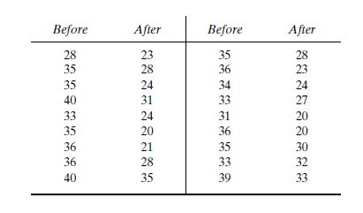
The speed ranges from 28 to 40 mi/h giving a speed range of 12. For five classes, the range per class is 2.4 mi/h. A frequency distribution table can then be prepared, as shown below in which the speed classes are listed in column 1 and the mid-values are in column 2. The number of observations for each class is listed in column 3 and the cumulative percentages of all observations are listed in column 6.
| 1 | 2 | 3 | 4 | 5 | 6 | 7 |
| Speed class (mi/h) | Class mid-value | Class frequency, | Percentage of class frequency | Cumulative percentage of class frequency | ||
| 28-30 | 29 | 4 | 116 | 13 | 13 | 139.24 |
| 31-33 | 32 | 5 | 160 | 17 | 30 | 42.05 |
| 34-36 | 35 | 12 | 420 | 40 | 70 | 0.12 |
| 37-39 | 38 | 6 | 228 | 20 | 90 | 57.66 |
| 40-42 | 41 | 3 | 123 | 10 | 100 | 111.63 |
| Total | 30 | 1047 | 350.7 |
Below Figure shows the frequency histogram for the data shown in above Table. The values in columns 2 and 3 of Table are used to draw the frequency histogram, where the abscissa represents the speeds and the ordinate the observed frequency in each class.

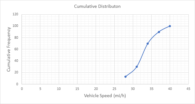
Below Figure shows the cumulative frequency distribution curve for the data given. In this case, the cumulative percentages in column 6 of above Table are plotted against the upper limit of each corresponding speed class. This curve gives the percentage of vehicles that are traveling at or below a given speed.

Determine the arithmetic mean speed:
After an increase in speed enforcement activities:
The speed ranges from 20 to 37 mi/h giving a speed range of 17. For six classes, the range per class is 2.83 mi/h. A frequency distribution table can then be prepared, as shown below in which the speed classes are listed in column 1 and the mid-values are in column 2. The number of observations for each class is listed in column 3 and the cumulative percentages of all observations are listed in column 6.
| 1 | 2 | 3 | 4 | 5 | 6 | 7 |
| Speed class (mi/h) | Class mid-value | Class frequency, | Percentage of class frequency | Cumulative percentage of class frequency | ||
| 20-22 | 21 | 6 | 126 | 20 | 20 | 253.5 |
| 23-25 | 24 | 8 | 192 | 27 | 47 | 98 |
| 26-28 | 27 | 4 | 108 | 13 | 60 | 1 |
| 29-31 | 30 | 3 | 90 | 10 | 70 | 18.75 |
| 32-34 | 33 | 5 | 165 | 17 | 87 | 151.25 |
| 35-37 | 36 | 4 | 144 | 13 | 100 | 289 |
| Total | 30 | 825 | 811.5 |
Below Figure shows the frequency histogram for the data shown in above Table. The values in columns 2 and 3 of Table are used to draw the frequency histogram, where the abscissa represents the speeds and the ordinate the observed frequency in each class.

Below Figure shows the cumulative frequency distribution curve for the data given. In this case, the cumulative percentages in column 6 of above Table are plotted against the upper limit of each corresponding speed class. This curve gives the percentage of vehicles that are traveling at or below a given speed.

Determine the arithmetic mean speed:
Conclusion:
The average speeds of each set of data are 34.9 and 27.5 mi/h respectively.
(b)
The histogram frequency distribution, cumulative percentage distribution for each set of data and 85th percentile speed.
Answer to Problem 10P
Explanation of Solution
Given:
Significance level of

Calculation:
Before an increase in speed enforcement activities:
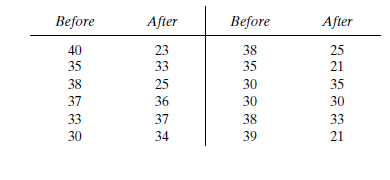
The speed ranges from 28 to 40 mi/h giving a speed range of 12. For five classes, the range per class is 2.4 mi/h. A frequency distribution table can then be prepared, as shown below in which the speed classes are listed in column 1 and the mid-values are in column 2. The number of observations for each class is listed in column 3 and the cumulative percentages of all observations are listed in column 6.
| 1 | 2 | 3 | 4 | 5 | 6 | 7 |
| Speed class (mi/h) | Class mid-value | Class frequency, | Percentage of class frequency | Cumulative percentage of class frequency | ||
| 28-30 | 29 | 4 | 116 | 13 | 13 | 139.24 |
| 31-33 | 32 | 5 | 160 | 17 | 30 | 42.05 |
| 34-36 | 35 | 12 | 420 | 40 | 70 | 0.12 |
| 37-39 | 38 | 6 | 228 | 20 | 90 | 57.66 |
| 40-42 | 41 | 3 | 123 | 10 | 100 | 111.63 |
| Total | 30 | 1047 | 350.7 |
Below Figure shows the frequency histogram for the data shown in above Table. The values in columns 2 and 3 of Table are used to draw the frequency histogram, where the abscissa represents the speeds and the ordinate the observed frequency in each class.

Below Figure shows the cumulative frequency distribution curve for the data given. In this case, the cumulative percentages in column 6 of above Table are plotted against the upper limit of each corresponding speed class. This curve gives the percentage of vehicles that are traveling at or below a given speed.

The 85th-percentile speed is obtained from the cumulative frequency distribution curve as 36 mi/h.
After an increase in speed enforcement activities:
The speed ranges from 20 to 37 mi/h giving a speed range of 17. For six classes, the range per class is 2.83 mi/h. A frequency distribution table can then be prepared, as shown below in which the speed classes are listed in column 1 and the mid-values are in column 2. The number of observations for each class is listed in column 3 and the cumulative percentages of all observations are listed in column 6.
| 1 | 2 | 3 | 4 | 5 | 6 | 7 |
| Speed class (mi/h) | Class mid-value | Class frequency, | Percentage of class frequency | Cumulative percentage of class frequency | ||
| 20-22 | 21 | 6 | 126 | 20 | 20 | 253.5 |
| 23-25 | 24 | 8 | 192 | 27 | 47 | 98 |
| 26-28 | 27 | 4 | 108 | 13 | 60 | 1 |
| 29-31 | 30 | 3 | 90 | 10 | 70 | 18.75 |
| 32-34 | 33 | 5 | 165 | 17 | 87 | 151.25 |
| 35-37 | 36 | 4 | 144 | 13 | 100 | 289 |
| Total | 30 | 825 | 811.5 |
Below Figure shows the frequency histogram for the data shown in above Table. The values in columns 2 and 3 of Table are used to draw the frequency histogram, where the abscissa represents the speeds and the ordinate the observed frequency in each class.

Below Figure shows the cumulative frequency distribution curve for the data given. In this case, the cumulative percentages in column 6 of above Table are plotted against the upper limit of each corresponding speed class. This curve gives the percentage of vehicles that are traveling at or below a given speed.

The 85th-percentile speed is obtained from the cumulative frequency distribution curve as 31.5 mi/h.
Conclusion:
The 85th-percentile speed for each set of data are 36 and 31.5 mi/h respectively.
(c)
The histogram frequency distribution, cumulative percentage distribution for each set of data and 15th percentile speed.
Answer to Problem 10P
Explanation of Solution
Given:
Significance level of


Calculation:
Before an increase in speed enforcement activities:
The speed ranges from 28 to 40 mi/h giving a speed range of 12. For five classes, the range per class is 2.4 mi/h. A frequency distribution table can then be prepared, as shown below in which the speed classes are listed in column 1 and the mid-values are in column 2. The number of observations for each class is listed in column 3 and the cumulative percentages of all observations are listed in column 6.
| 1 | 2 | 3 | 4 | 5 | 6 | 7 |
| Speed class (mi/h) | Class mid-value | Class frequency, | Percentage of class frequency | Cumulative percentage of class frequency | ||
| 28-30 | 29 | 4 | 116 | 13 | 13 | 139.24 |
| 31-33 | 32 | 5 | 160 | 17 | 30 | 42.05 |
| 34-36 | 35 | 12 | 420 | 40 | 70 | 0.12 |
| 37-39 | 38 | 6 | 228 | 20 | 90 | 57.66 |
| 40-42 | 41 | 3 | 123 | 10 | 100 | 111.63 |
| Total | 30 | 1047 | 350.7 |
Below Figure shows the frequency histogram for the data shown in above Table. The values in columns 2 and 3 of Table are used to draw the frequency histogram, where the abscissa represents the speeds and the ordinate the observed frequency in each class.
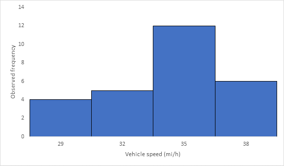
Below Figure shows the cumulative frequency distribution curve for the data given. In this case, the cumulative percentages in column 6 of above Table are plotted against the upper limit of each corresponding speed class. This curve gives the percentage of vehicles that are traveling at or below a given speed.

The 15th-percentile speed is obtained from the cumulative frequency distribution curve as 28.5 mi/h.
After an increase in speed enforcement activities:
The speed ranges from 20 to 37 mi/h giving a speed range of 17. For six classes, the range per class is 2.83 mi/h. A frequency distribution table can then be prepared, as shown below in which the speed classes are listed in column 1 and the mid-values are in column 2. The number of observations for each class is listed in column 3 and the cumulative percentages of all observations are listed in column 6.
| 1 | 2 | 3 | 4 | 5 | 6 | 7 |
| Speed class (mi/h) | Class mid-value | Class frequency, | Percentage of class frequency | Cumulative percentage of class frequency | ||
| 20-22 | 21 | 6 | 126 | 20 | 20 | 253.5 |
| 23-25 | 24 | 8 | 192 | 27 | 47 | 98 |
| 26-28 | 27 | 4 | 108 | 13 | 60 | 1 |
| 29-31 | 30 | 3 | 90 | 10 | 70 | 18.75 |
| 32-34 | 33 | 5 | 165 | 17 | 87 | 151.25 |
| 35-37 | 36 | 4 | 144 | 13 | 100 | 289 |
| Total | 30 | 825 | 811.5 |
Below Figure shows the frequency histogram for the data shown in above Table. The values in columns 2 and 3 of Table are used to draw the frequency histogram, where the abscissa represents the speeds and the ordinate the observed frequency in each class.
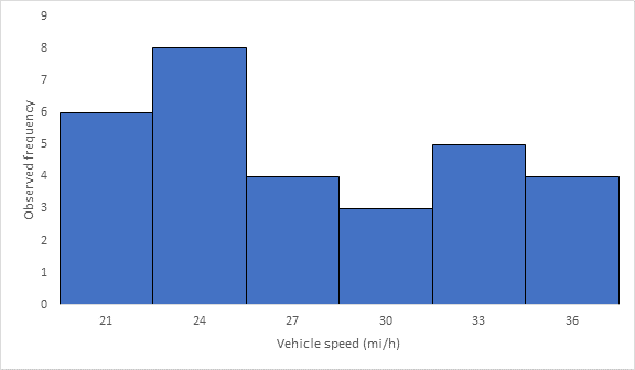
Below Figure shows the cumulative frequency distribution curve for the data given. In this case, the cumulative percentages in column 6 of above Table are plotted against the upper limit of each corresponding speed class. This curve gives the percentage of vehicles that are traveling at or below a given speed.
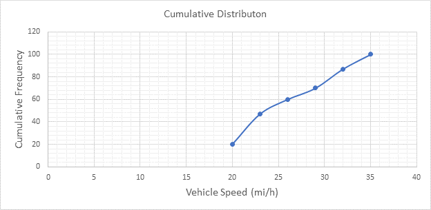
The 15th-percentile speed is obtained from the cumulative frequency distribution curve as 0 mi/h.
Conclusion:
The 15th-percentile speed for each set of data are 28.5 and 0 mi/h respectively.
(d)
The histogram frequency distribution, cumulative percentage distribution for each set of data and mode.
Answer to Problem 10P
35 mi/h and 24 mi/h
Explanation of Solution
Given:
Significance level of


Calculation:
Before an increase in speed enforcement activities:
The speed ranges from 28 to 40 mi/h giving a speed range of 12. For five classes, the range per class is 2.4 mi/h. A frequency distribution table can then be prepared, as shown below in which the speed classes are listed in column 1 and the mid-values are in column 2. The number of observations for each class is listed in column 3 and the cumulative percentages of all observations are listed in column 6.
| 1 | 2 | 3 | 4 | 5 | 6 | 7 |
| Speed class (mi/h) | Class mid-value | Class frequency, | Percentage of class frequency | Cumulative percentage of class frequency | ||
| 28-30 | 29 | 4 | 116 | 13 | 13 | 139.24 |
| 31-33 | 32 | 5 | 160 | 17 | 30 | 42.05 |
| 34-36 | 35 | 12 | 420 | 40 | 70 | 0.12 |
| 37-39 | 38 | 6 | 228 | 20 | 90 | 57.66 |
| 40-42 | 41 | 3 | 123 | 10 | 100 | 111.63 |
| Total | 30 | 1047 | 350.7 |
Below Figure shows the frequency histogram for the data shown in above Table. The values in columns 2 and 3 of Table are used to draw the frequency histogram, where the abscissa represents the speeds and the ordinate the observed frequency in each class.

Below Figure shows the cumulative frequency distribution curve for the data given. In this case, the cumulative percentages in column 6 of above Table are plotted against the upper limit of each corresponding speed class. This curve gives the percentage of vehicles that are traveling at or below a given speed.

The mode or modal speed is obtained from the frequency histogram as 35 mi/h
After an increase in speed enforcement activities:
The speed ranges from 20 to 37 mi/h giving a speed range of 17. For six classes, the range per class is 2.83 mi/h. A frequency distribution table can then be prepared, as shown below in which the speed classes are listed in column 1 and the mid-values are in column 2. The number of observations for each class is listed in column 3 and the cumulative percentages of all observations are listed in column 6.
| 1 | 2 | 3 | 4 | 5 | 6 | 7 |
| Speed class (mi/h) | Class mid-value | Class frequency, | Percentage of class frequency | Cumulative percentage of class frequency | ||
| 20-22 | 21 | 6 | 126 | 20 | 20 | 253.5 |
| 23-25 | 24 | 8 | 192 | 27 | 47 | 98 |
| 26-28 | 27 | 4 | 108 | 13 | 60 | 1 |
| 29-31 | 30 | 3 | 90 | 10 | 70 | 18.75 |
| 32-34 | 33 | 5 | 165 | 17 | 87 | 151.25 |
| 35-37 | 36 | 4 | 144 | 13 | 100 | 289 |
| Total | 30 | 825 | 811.5 |
Below Figure shows the frequency histogram for the data shown in above Table. The values in columns 2 and 3 of Table are used to draw the frequency histogram, where the abscissa represents the speeds and the ordinate the observed frequency in each class.

Below Figure shows the cumulative frequency distribution curve for the data given. In this case, the cumulative percentages in column 6 of above Table are plotted against the upper limit of each corresponding speed class. This curve gives the percentage of vehicles that are traveling at or below a given speed.

The mode or modal speed is obtained from the frequency histogram as 24 mi/h.
Conclusion:
The mode for each set of data are 35 and 24 mi/h respectively.
(e)
The histogram frequency distribution, cumulative percentage distribution for each set of data and median.
Answer to Problem 10P
32.5 and 23.5 mi/h
Explanation of Solution
Given:
Significance level of


Calculation:
Before an increase in speed enforcement activities:
The speed ranges from 28 to 40 mi/h giving a speed range of 12. For five classes, the range per class is 2.4 mi/h. A frequency distribution table can then be prepared, as shown below in which the speed classes are listed in column 1 and the mid-values are in column 2. The number of observations for each class is listed in column 3 and the cumulative percentages of all observations are listed in column 6.
| 1 | 2 | 3 | 4 | 5 | 6 | 7 |
| Speed class (mi/h) | Class mid-value | Class frequency, | Percentage of class frequency | Cumulative percentage of class frequency | ||
| 28-30 | 29 | 4 | 116 | 13 | 13 | 139.24 |
| 31-33 | 32 | 5 | 160 | 17 | 30 | 42.05 |
| 34-36 | 35 | 12 | 420 | 40 | 70 | 0.12 |
| 37-39 | 38 | 6 | 228 | 20 | 90 | 57.66 |
| 40-42 | 41 | 3 | 123 | 10 | 100 | 111.63 |
| Total | 30 | 1047 | 350.7 |
Below Figure shows the frequency histogram for the data shown in above Table. The values in columns 2 and 3 of Table are used to draw the frequency histogram, where the abscissa represents the speeds and the ordinate the observed frequency in each class.

Below Figure shows the cumulative frequency distribution curve for the data given. In this case, the cumulative percentages in column 6 of above Table are plotted against the upper limit of each corresponding speed class. This curve gives the percentage of vehicles that are traveling at or below a given speed.

The median speed is obtained from the cumulative frequency distribution curve as 32.5 mi/h which is the 50th percentile speed.
After an increase in speed enforcement activities:
The speed ranges from 20 to 37 mi/h giving a speed range of 17. For six classes, the range per class is 2.83 mi/h. A frequency distribution table can then be prepared, as shown below in which the speed classes are listed in column 1 and the mid-values are in column 2. The number of observations for each class is listed in column 3 and the cumulative percentages of all observations are listed in column 6.
| 1 | 2 | 3 | 4 | 5 | 6 | 7 |
| Speed class (mi/h) | Class mid-value | Class frequency, | Percentage of class frequency | Cumulative percentage of class frequency | ||
| 20-22 | 21 | 6 | 126 | 20 | 20 | 253.5 |
| 23-25 | 24 | 8 | 192 | 27 | 47 | 98 |
| 26-28 | 27 | 4 | 108 | 13 | 60 | 1 |
| 29-31 | 30 | 3 | 90 | 10 | 70 | 18.75 |
| 32-34 | 33 | 5 | 165 | 17 | 87 | 151.25 |
| 35-37 | 36 | 4 | 144 | 13 | 100 | 289 |
| Total | 30 | 825 | 811.5 |
Below Figure shows the frequency histogram for the data shown in above Table. The values in columns 2 and 3 of Table are used to draw the frequency histogram, where the abscissa represents the speeds and the ordinate the observed frequency in each class.

Below Figure shows the cumulative frequency distribution curve for the data given. In this case, the cumulative percentages in column 6 of above Table are plotted against the upper limit of each corresponding speed class. This curve gives the percentage of vehicles that are traveling at or below a given speed.

The median speed is obtained from the cumulative frequency distribution curve as 23.5 mi/h which is the 50th percentile speed.
Conclusion:
The median speed for each set of data are 32.5 and 23.5 mi/h respectively.
(f)
The histogram frequency distribution, cumulative percentage distribution for each set of data and pace.
Answer to Problem 10P
32 to 39 mi/h and 27 to 36 mi/h
Explanation of Solution
Given:
Significance level of


Calculation:
Before an increase in speed enforcement activities:
The speed ranges from 28 to 40 mi/h giving a speed range of 12. For five classes, the range per class is 2.4 mi/h. A frequency distribution table can then be prepared, as shown below in which the speed classes are listed in column 1 and the mid-values are in column 2. The number of observations for each class is listed in column 3 and the cumulative percentages of all observations are listed in column 6.
| 1 | 2 | 3 | 4 | 5 | 6 | 7 |
| Speed class (mi/h) | Class mid-value | Class frequency, | Percentage of class frequency | Cumulative percentage of class frequency | ||
| 28-30 | 29 | 4 | 116 | 13 | 13 | 139.24 |
| 31-33 | 32 | 5 | 160 | 17 | 30 | 42.05 |
| 34-36 | 35 | 12 | 420 | 40 | 70 | 0.12 |
| 37-39 | 38 | 6 | 228 | 20 | 90 | 57.66 |
| 40-42 | 41 | 3 | 123 | 10 | 100 | 111.63 |
| Total | 30 | 1047 | 350.7 |
Below Figure shows the frequency histogram for the data shown in above Table. The values in columns 2 and 3 of Table are used to draw the frequency histogram, where the abscissa represents the speeds and the ordinate the observed frequency in each class.

Below Figure shows the cumulative frequency distribution curve for the data given. In this case, the cumulative percentages in column 6 of above Table are plotted against the upper limit of each corresponding speed class. This curve gives the percentage of vehicles that are traveling at or below a given speed.
Below figure shows the frequency distribution curve for the data given. In this case, a curve showing percentage of observations against speed is drawn by plotting values from column 5 of above Table against the corresponding values in column 2. The total area under this curve is one or 100 percent.
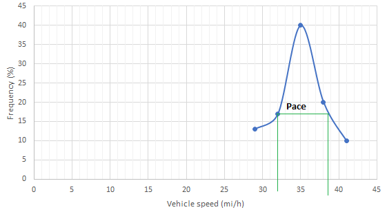
The pace is obtained from the frequency distribution curve above as 32 to 39 mi/h.
After an increase in speed enforcement activities:
The speed ranges from 20 to 37 mi/h giving a speed range of 17. For six classes, the range per class is 2.83 mi/h. A frequency distribution table can then be prepared, as shown below in which the speed classes are listed in column 1 and the mid-values are in column 2. The number of observations for each class is listed in column 3 and the cumulative percentages of all observations are listed in column 6.
| 1 | 2 | 3 | 4 | 5 | 6 | 7 |
| Speed class (mi/h) | Class mid-value | Class frequency, | Percentage of class frequency | Cumulative percentage of class frequency | ||
| 20-22 | 21 | 6 | 126 | 20 | 20 | 253.5 |
| 23-25 | 24 | 8 | 192 | 27 | 47 | 98 |
| 26-28 | 27 | 4 | 108 | 13 | 60 | 1 |
| 29-31 | 30 | 3 | 90 | 10 | 70 | 18.75 |
| 32-34 | 33 | 5 | 165 | 17 | 87 | 151.25 |
| 35-37 | 36 | 4 | 144 | 13 | 100 | 289 |
| Total | 30 | 825 | 811.5 |
Below Figure shows the frequency histogram for the data shown in above Table. The values in columns 2 and 3 of Table are used to draw the frequency histogram, where the abscissa represents the speeds and the ordinate the observed frequency in each class.

Below Figure shows the cumulative frequency distribution curve for the data given. In this case, the cumulative percentages in column 6 of above Table are plotted against the upper limit of each corresponding speed class. This curve gives the percentage of vehicles that are traveling at or below a given speed.

Below figure shows the frequency distribution curve for the data given. In this case, a curve showing percentage of observations against speed is drawn by plotting values from column 5 of above Table against the corresponding values in column 2. The total area under this curve is one or 100 percent.
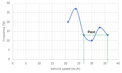
The pace is obtained from the frequency distribution curve drawn above as 27 to 36 mi/h.
Conclusion:
The pace for each set of data are 32 to 39 mi/h and 27 to 36 mi/h respectively.
Want to see more full solutions like this?
Chapter 4 Solutions
Traffic and Highway Engineering
- q.complete. Answer.arrow_forwardhello can i get some help please?arrow_forwardThe results of the travel time study are summarized in the following table. For this data: a. Tabulate and graphically present travel time and delay results. b. Show the average travel speed and average running speed for each section.arrow_forward
- Example: For the given spot speed data, conduct the following: 1. Plot the frequency and cumulative frequency distribution of the speed data. 2. Calculate the: Average Speed , Median Speed and Modal Speed, The pace and the percent of vehicle in pace and Standard deviation and estimated standard deviation. Speed (kph) Frequency of Vehicles(n) 81.6 86.6 1 89.3 2 92.2 4 95.2 8 98.5 10 102 13 105.8 15 109.9 11 114.3 8 119 124.2 1 129.9arrow_forwardThe vehicle count obtained in every 10-minute interval of a traffic volume survey done in peak one hour is given below. Time Interval (in minutes) 0-10 10-20 20-30 30-40 40-50 50-60 Vehicle Count 10 11 12 15 13 11 The peak hour factor (PHF) for 10 minute sub-interval is off to one decimal place) (roundarrow_forwardGiven the following spot speed data: Speed Group Observed vehicles 45-49 5 50-53 16 54-57 29 58-61 36 62-65 41 66-69 21 70-73 4 A. Calculate the 15th, 50th, and 85th percentile. B. Recommend appropriate speed limits with justification.arrow_forward
- Given the following data: The route will use 40-seat standard buses The door opening and closing time is 4 seconds The boarding time is 3.5 seconds and 4.0 seconds for standing passengers The alighting time is 2 seconds Use the attached table to calculate the average dwell time of the bus at each of the 10 stationsarrow_forwardHelp me urgent... Thank youarrow_forward5-4.. The following traffic count data were taken from a per- manent detector location on a major state highway. 1. 2. 3. 4. 5. Month No. of Total Total Total Weekdays Days in Monthly Weekday Volume in Month Month Volume (days) (days) (vehs) (vehs) 200,000 210,000 215,000 205,000 195,000 193,000 180,000 175,000 189,000 170,000 171,000 Jan 22 31 Feb 20 28 185,000 180,000: 172,000 168,000 160,000 150,000 -175,000 178,000 182,000 176,000 Mar 22 31 30 Apr May Jun 22 21 31 22 30 Jul 23 31 21 31 Aug Sep Oct 22 30 198,000 205,000 200,000 22 31 Nov 21 30 Dec 22 31 From this data, determine (a) the AADT, (b) the ADT for each month, (c) the AAWT, and (d) the AWT for each month. From this information, what can be dis- cerned about the character of the facility and the demand it serves?arrow_forward
- The spot speed data on the corridor was collected as shown in the Table below. Vehicle # Spot speed (mph) 1 2 3 4 45 45 45 40 If X is the value of time-mean speed, and Y is the value of space-mean speed. Then, report the value of X minus Y, correct to 1 digit after the decimal.arrow_forwardConsider the following plot of cumulative arriving and departing vehicles at a freeway bottleneck location: Vehicles 20,000 15,000 10,000 5,000 0 0 30 60 90 120 150 180 210 240 270 300 330 360 Time (mins) Arrivals (vehs) Departures (vehs) From this plot, determine the following: A. What is the capacity of the bottleneck location? 9000 whole number, i.e. X000.) B. What is the maximum size of the queue that develops? 3250 whole number, i.e. X000.) C. What is the longest wait time that any vehicle experiences during the breakdown? to the nearest whole number, i.e. XX.) (Hint: Provide the answer as a numerical number only in units of vehicles per hour and rounded to the nearest thousand (Hint: Provide the answer as a numerical number only in units of vehicles and rounded to the nearest thousand (Hint: Provide the answer as a numerical number only in units of minutes and roundedarrow_forwardaqsqarrow_forward
 Traffic and Highway EngineeringCivil EngineeringISBN:9781305156241Author:Garber, Nicholas J.Publisher:Cengage Learning
