
Videos
Going extinct. A paleontologist has gathered data on fossils for a certain species of brachiopods. This species is now extinct and the scientist wants to estimate when this extinction occurred. A total of nine fossils have been discovered and dated as shown in the table below. (These data are estimated from the work of Y.G. Jin et at, “Patterns of Marine Mass Extinction,” Science,
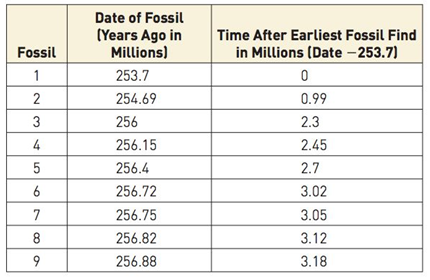
Using each of the five methods described in the text to count tanks, compute five estimates of the date around which this species went extinct. (Use the data in the far right column of the table, then convert your answers to a date millions of years ago.) Which estimate do you think is the best? Why?
Want to see the full answer?
Check out a sample textbook solution
Chapter 9 Solutions
The Heart of Mathematics: An Invitation to Effective Thinking
Additional Math Textbook Solutions
Probability and Statistics for Engineers and Scientists
Mathematics with Applications In the Management, Natural, and Social Sciences (12th Edition)
Using & Understanding Mathematics: A Quantitative Reasoning Approach (7th Edition)
Mathematical Methods in the Physical Sciences
A Problem Solving Approach to Mathematics for Elementary School Teachers (12th Edition)
Finite Mathematics & Its Applications (12th Edition)


- Urban Travel Times Population of cities and driving times are related, as shown in the accompanying table, which shows the 1960 population N, in thousands, for several cities, together with the average time T, in minutes, sent by residents driving to work. City Population N Driving time T Los Angeles 6489 16.8 Pittsburgh 1804 12.6 Washington 1808 14.3 Hutchinson 38 6.1 Nashville 347 10.8 Tallahassee 48 7.3 An analysis of these data, along with data from 17 other cities in the United States and Canada, led to a power model of average driving time as a function of population. a Construct a power model of driving time in minutes as a function of population measured in thousands b Is average driving time in Pittsburgh more or less than would be expected from its population? c If you wish to move to a smaller city to reduce your average driving time to work by 25, how much smaller should the city be?arrow_forwardThe Great White Shark. In an article titled “Great White, Deep Trouble” (National Geographic, Vol. 197(4), pp. 2–29), Peter Benchley—the author of JAWS—discussed various aspects of the Great White Shark (Carcharodon carcharias). Data on the number of pups borne in a lifetime by each of 80 Great White Shark females are provided on the WeissStats site. a. obtain and interpret the quartiles. b. determine and interpret the interquartile range. c. find and interpret the five-number summary. d. identify potential outliers, if any. e. obtain and interpret a boxplot.arrow_forward2.86 Shaft graves in ancient Greece. Refer to the American O Journal of Archaeology (Jan. 2014) study of sword shaft SHAFTS graves in ancient Greece, Exercise 2.60 (p. 61). The num- ber of sword shafts buried at each of 13 recently discovered grave sites is reproduced in the following table. 1 2 3 1 5 6 2 4 1 2 4 2 9 Source: Harrell, K. "The fallen and their swords: A new explanation for the rise of the shaft graves." American Journal of Archaeology, Vol. 118, No. 1, January 2014 (Figure 1). a. Calculate the range of the sample data. b. Calculate the variance of the sample data. c. Calculate the standard deviation of the sample data.arrow_forward
- A certain species of tree has an average life span of 130 years. A researcher has noticed a large number of trees of this species washing up along a beach as driftwood. She takes core samples from 27 of those trees to count the number of rings and measure the widths of the rings. Counting the rings allows the researcher to determine the age of each tree. Her data are displayed in the provided table. One of her interests is determining if this sample provides evidence that the average age of the driftwood is less than the 130 year life span expected for this type of tree. If the average age is less than 130 years it might suggest that the trees have died from unusual causes, such as invasive beetles or logging. 127 98 79 147 200 130 60 51 81 98 160 165 134 62 152 66 Reference: 4-8-Technology 105 75 120 113 200 190 68 124 190 159 60 Describe how you would generate a single randomization sample in this situation, and identify the statistic you would calculate for each sample.arrow_forwardA cohort study is conducted to assess the association between hypertension and the risk of stroke. The study involves n=1,250 participants who are free of stroke at the study start. Each participant is assessed at study start (baseline) and every year thereafter for five years. The following table displays data on hypertension status measured at baseline and hypertension status measured two years later. 2 Years: Not Hypertensive 2 Years: Hypertensive Baseline: Not Hypertensive 850 148 Baseline: Hypertensive 45 207 Compute the cumulative incidence of hypertension over 2 years. Group of answer choices 17.1%arrow_forward6 A study was conducted that measured the total brain volume (TBV) (in mm3) of patients that had schizophrenia and patients that are considered normal. Table #1 contains the TBV of the normal patients and Table #2 contains the TBV of schizophrenia patients ("SOCR data Oct2009," 2013). Table #1: Total Brain Volume (in mm3) of Normal Patients 1663407 1583940 1299470 1535137 1431890 1578698 1453510 1650348 1288971 1366346 1326402 1503005 1474790 1317156 1441045 1463498 1650207 1523045 1441636 1432033 1420416 1480171 1360810 1410213 1574808 1502702 1203344 1319737 1688990 1292641 1512571 1635918 Table #2: Total Brain Volume (in mm3) of Schizophrenia Patients 1331777 1487886 1066075 1297327 1499983 1861991 1368378 1476891 1443775 1337827 1658258 1588132 1690182 1569413 1177002 1387893 1483763 1688950 1563593 1317885 1420249 1363859 1238979…arrow_forward
- 6B A study was conducted that measured the total brain volume (TBV) (in mm3) of patients that had schizophrenia and patients that are considered normal. Table #1 contains the TBV of the normal patients and Table #2 contains the TBV of schizophrenia patients ("SOCR data Oct2009," 2013). Table #1: Total Brain Volume (in mm3) of Normal Patients 1663407 1583940 1299470 1535137 1431890 1578698 1453510 1650348 1288971 1366346 1326402 1503005 1474790 1317156 1441045 1463498 1650207 1523045 1441636 1432033 1420416 1480171 1360810 1410213 1574808 1502702 1203344 1319737 1688990 1292641 1512571 1635918 Table #2: Total Brain Volume (in mm3) of Schizophrenia Patients 1331777 1487886 1066075 1297327 1499983 1861991 1368378 1476891 1443775 1337827 1658258 1588132 1690182 1569413 1177002 1387893 1483763 1688950 1563593 1317885 1420249 1363859 1238979…arrow_forwardThe Journal of Engineering in Industry (Aug. 1993) reported on an automated system designed to replace the cutting tool of a drilling machine at optimum times. To test the system, data were collected over a broad range of materials, drill sizes, drill speeds, and feed rates – called machining conditions. Although a total of 168 different machining conditions were possible, only eight were employed in this study. These are described below: Experiment Workpiece Drill Size (in.) 25 25 Drill Speed (грт) 1250 1800 Feed Rate Material (ipr) .011 .005 1 Cast Iron Cast Iron Steel Steel 25 25 3750 2500 .003 .003 .008 4 Steel 25 .125 .125 2500 Steel Steel 4000 4000 3000 .0065 .009 .010 Steel .125 a. Suppose one (and only one) of the 168 possible machining conditions will detect a flaw in the system. What is the probability that the experiment conducted in the study will detect the system flaw? b. Suppose the system flaw occurs when drilling steel material with a 25-inch drill size at a speed of…arrow_forwardMeteoroids. In the article “Interstellar Pelting” (Scientific American, Vol. 288, No. 5, pp. 28–30), G. Musser explained that information on extrasolar planets can be discerned from foreign material and dust found in our solar system. Studies show that 1 in every 100 meteoroids entering Earth’s atmosphere is actually alien matter from outside our solar system. a. Of 300 meteoroids entering the Earth’s atmosphere, how many would you expect to be alien matter from outside our solar system? Justify your answer. b. Apply the Poisson approximation to the binomial distribution to determine the probability that, of 300 meteoroids entering the Earth’s atmosphere, between 2 and 4, inclusive, are alien matter from outside our solar system. c. Apply the Poisson approximation to the binomial distribution to determine the probability that, of 300 meteoroids entering the Earth’s atmosphere, at least 1 is alien matter from outside our solar system.arrow_forward
- The article "Oxidation State and Activities of Chromium Oxides in Cao-SiO,-CrO, Slag System" (Y. Xiao, L. Holappa, and M. Reuter, Metallurgical and Materials Transactions B, 2002:595-603) presents the amount x (in mole percent) and activity coefficient y of CrO,5 for several specimens. The data, extracted from a larger table, are presented in the following table. х У 2.6 10.20 5.03 19.9 8.84 0.8 6.62 5.3 2.89 20.3 2.31 39.4 7.13 5.8 3.40 29.4 5.57 2.2 7.23 5.5 2.12 33.1 1.67 44.2 5.33 13.1 16.70 0.6 9.75 2.2 2.74 16.9 2.58 35.5 1.50 48.0 Compute the least-squares line for predicting y from x. b. Plot the residuals versus the fitted values. Compute the least-squares line for predicting y from 1/x. d. Plot the residuals versus the fitted values. C. Using the better fitting line, find a 95% confidence interval for the mean value of y when x= 5.0.arrow_forwardThe article "Estimating Population Abundance in Plant Species with Dormant Life-Stages: Fire and the Endangered Plant Grevillea caleye R Br." (T. Auld and J. Scott, Ecological Management and Restoration, 2004:125-129) presents estimates of population sizes of a certain rare shrub in areas burnt by fire. The following table presents population counts and areas (in m?) for several patches containing the plant. Агеа 3739 Population 3015 5277 1847 400 17 345 392 142 40 7000 2521 213 11958 1200 2878 707 113 1392 157 12000 10880 711 74 2259 223 81 15 33 18 1254 1320 229 351 1000 92 841 1720 1500 300 228 31 228 17 10 Compute the least-squares line for predicting population (y) from area (x). Б. a. Plot the residuals versus the fitted values. Does the model seem appropriate? Compute the least-squares line for predicting In y from In x. Plot the residuals versus the fitted values. Does the model seem appropriate? Using the more appropriate model, construct a 95% prediction interval for the…arrow_forwardThe following table shows the typical depth (rounded to the nearest foot) for nonfailed wells in geological formations in Baltimore County (The Journal of Data Science, 2009, Vol. 7, pp. 111-127). Geological Formation Group Number of Nonfailed Wells Nonfailed Well Depth Gneiss 1,515 255 Granite 26 218 Loch Raven Schist 3,290 317 Mafic 349 231 Marble 280 267 Prettyboy Schist 1,343 255 Other schists 887 267 Serpentine 36 217 Total 7,726 2,027 Let the random variable X denote the depth (rounded to the nearest foot) for nonfailed wells. Detemine the cumulative distribution function for X. Round your answers to four decimal places (e.g. 98.7654). x < 217 217arrow_forwardarrow_back_iosSEE MORE QUESTIONSarrow_forward_ios
 Functions and Change: A Modeling Approach to Coll...AlgebraISBN:9781337111348Author:Bruce Crauder, Benny Evans, Alan NoellPublisher:Cengage Learning
 Linear Algebra: A Modern IntroductionAlgebraISBN:9781285463247Author:David PoolePublisher:Cengage Learning
 Calculus For The Life SciencesCalculusISBN:9780321964038Author:GREENWELL, Raymond N., RITCHEY, Nathan P., Lial, Margaret L.Publisher:Pearson Addison Wesley,
 Glencoe Algebra 1, Student Edition, 9780079039897...AlgebraISBN:9780079039897Author:CarterPublisher:McGraw Hill