Concept explainers
19
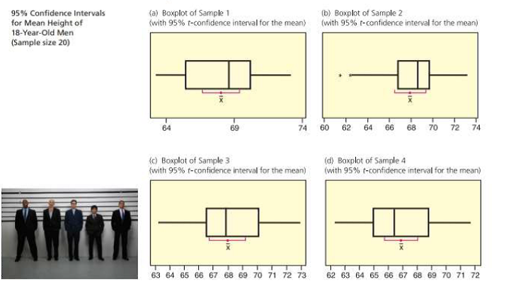
Critical Thinking: Boxplots and Confidence Intervals The distribution of heights of 18-year-old men in the United States is approximately normal. with
| VARIABLE | N | MEAN | STDEV | SEMEAN | 95.0 | % CI |
| Sample 1 | 20 | 68.050 | 2.901 | 0.649 | 69.407) | |
| Sample a | 20 | 67.956 | 3.137 | 0.702 | (66.490 | 69.426 |
| Sample 3 | 20 | 67.976 | 2.639 | 0.590 | (66.741 , | 69.211) |
| Sample 4 | 20 | 66.908 | 2.440 | 0.546 | (65.766 , | 68.050) |
(a) Examine the figure (parts (a) to (d)). How do the boxplots for the four samples differ? Why should you expect the boxplots to differ ?

(b) Examine the 95% confidence intervals for the four sample shown in the printout. Do the intervals differ in length? Do the intervals all contain the expected population mean of tot inches? If we draw more samples, do you expect all of the resulting 95% confidence intervals to contain µ = 68 ? Why or why not?
Trending nowThis is a popular solution!

Chapter 8 Solutions
Understanding Basic Statistics
- Exercise 4.2 Prove that, if A and B are independent, then so are A and B, Ac and B, and A and B.arrow_forward8. Show that, if {Xn, n ≥ 1) are independent random variables, then sup X A) < ∞ for some A.arrow_forward8- 6. Show that, for any random variable, X, and a > 0, 8 心 P(xarrow_forward15. This problem extends Problem 20.6. Let X, Y be random variables with finite mean. Show that 00 (P(X ≤ x ≤ Y) - P(X ≤ x ≤ X))dx = E Y — E X.arrow_forward(b) Define a simple random variable. Provide an example.arrow_forward17. (a) Define the distribution of a random variable X. (b) Define the distribution function of a random variable X. (c) State the properties of a distribution function. (d) Explain the difference between the distribution and the distribution function of X.arrow_forward16. (a) Show that IA(w) is a random variable if and only if A E Farrow_forward15. Let 2 {1, 2,..., 6} and Fo({1, 2, 3, 4), (3, 4, 5, 6}). (a) Is the function X (w) = 21(3, 4) (w)+711.2,5,6) (w) a random variable? Explain. (b) Provide a function from 2 to R that is not a random variable with respect to (N, F). (c) Write the distribution of X. (d) Write and plot the distribution function of X.arrow_forward20. Define the o-field R2. Explain its relation to the o-field R.arrow_forward7. Show that An → A as n→∞ I{An} - → I{A} as n→ ∞.arrow_forward7. (a) Show that if A,, is an increasing sequence of measurable sets with limit A = Un An, then P(A) is an increasing sequence converging to P(A). (b) Repeat the same for a decreasing sequence. (c) Show that the following inequalities hold: P (lim inf An) lim inf P(A) ≤ lim sup P(A) ≤ P(lim sup A). (d) Using the above inequalities, show that if A, A, then P(A) + P(A).arrow_forward19. (a) Define the joint distribution and joint distribution function of a bivariate ran- dom variable. (b) Define its marginal distributions and marginal distribution functions. (c) Explain how to compute the marginal distribution functions from the joint distribution function.arrow_forwardarrow_back_iosSEE MORE QUESTIONSarrow_forward_ios
 Glencoe Algebra 1, Student Edition, 9780079039897...AlgebraISBN:9780079039897Author:CarterPublisher:McGraw Hill
 Holt Mcdougal Larson Pre-algebra: Student Edition...AlgebraISBN:9780547587776Author:HOLT MCDOUGALPublisher:HOLT MCDOUGAL
 Big Ideas Math A Bridge To Success Algebra 1: Stu...AlgebraISBN:9781680331141Author:HOUGHTON MIFFLIN HARCOURTPublisher:Houghton Mifflin Harcourt


