Concept explainers
Videos
a.
Find the equation of the least-squares line, if y is expressed in kilograms instead of pounds.
a.
Answer to Problem 28E
The equation of the least-squares line, if y is expressed in kilograms instead of pounds is
Explanation of Solution
Calculation:
The least-squares regression equation relating the shear strength (pounds or lb), y of steel to weld diameter, x is given as
Data transformation:
Software procedure:
Step-by-step procedure to transform the data using the MINITAB software:
- Choose Calc > Calculator.
- Enter the column of y1 under Store result in variable.
- Enter the 0.4536*‘y’ in Expression.
- Click OK in all dialogue boxes.
The transformed data, where each
The least-squares equation can be obtained using software.
Least-squares equation:
Software procedure:
Step-by-step procedure to obtain the least-squares equation using the MINITAB software:
- Choose Stat > Regression > Regression > Fit Regression Model.
- Enter the column of y1 under Responses.
- Enter the column of x under Continuous predictors.
- Choose Results and select Coefficients, Regression Equation.
- Click OK in all dialogue boxes.
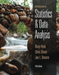
Output obtained using MINITAB is given below:
Thus, the equation of the least-squares line, if y is expressed in kilograms instead of pounds is
b.
Find the new slope, intercept, and equation of the least-squares line, if a constant, c is multiplied with every observation on y.
b.
Answer to Problem 28E
The new slope is –936.22 c.
The new intercept is 8.577 c.
The new equation of the least-squares line is
Explanation of Solution
Calculation:
Changing the unit of y from pounds to kilograms causes a change in the scale of y. Now, if the scale of the response variable in a regression, y, is changed by multiplying with a constant c, each least-squares coefficient is also multiplied by c.
Thus, each coefficient in the regression equation, that is, the intercept –936.22 and the slope corresponding to x, 8.577, will be multiplied by c, in order to get the regression equation in this situation. The regression equation is
Thus, the new slope is –936.22 c; the new intercept is 8.577 c; the new equation of the least-squares line is
These can be verified by using the formulae for a and b. The general formulae for a and b, for a simple least-squares regression equation,
Now,
Therefore,
Substitute the values of new a and newb in the general form of the regression equation.
In this problem, a = –936.22 and b = 8.577. As a result, the new slope is –936.22 c; the new intercept is 8.577 c.
Substituting these values in the equation for
Want to see more full solutions like this?
Chapter 5 Solutions
Introduction to Statistics and Data Analysis


- If your graphing calculator is capable of computing a least-squares sinusoidal regression model, use it to find a second model for the data. Graph this new equation along with your first model. How do they compare?arrow_forwardA photoconductor film is manufactured at a nominal thickness of 25 mils. The product engineer wishes to increase the mean speed of the film and believes that this can be achieved by reducing the thickness of the film to 20 mils. Eight samples of each film thickness are manufactured in a pilot production process, and the film speed (in microjoules per square inch) is measured. For the 25-mil film, the sample data result is.x₁ = 1.15 and S₁ = 0.11, while for the 20-mil film, the data yield 2 = 1.06 and s2 = 0.09. Note that an increase in film speed would lower the value of the observation in microjoules per square inch. Do the data support the claim that reducing the film thickness increases the mean speed of the film? Use a = 0.10 and assume that the two population variances are equal and the underlying population of film speed is normally distributed. The appropriate decision for the test is to reject the null hypothesis True Falsearrow_forwardMeasurements were taken against time to determine the temperature change along a wall. Using the least-squares method, describe the temperature change as a function of time with the data in the table.arrow_forward
- 6. Find the average value of city (2x - 1)³dx.arrow_forwardThe number of inches that a recently built structure sits on the ground is given by (image) where x is its age in months. Use the least squares method to estimate alpha.arrow_forwardA researcher collects data that represents the average number of hours of sleep in the last two nights by 8 depressed patients and 9 non-depressed patients. The researcher is interested in whether the two groups reliably differ in the amount of sleep they get. Use Jamovi to calculate t-obt and the p value.arrow_forward
- Given the “data” determined by y = x^3 + (x-1)^2 with x = 0.1, 1.2, 2.3, and 2.9, calculate SSTO, SSR, and R^2. Then recalculate these using x = 0.3, 1, 2.45, and 2.8. Does where you collect your data (i.e., which values of x) appear to impact your interpretation of how good the linear model fits?.arrow_forwardSuppose the manager of a gas station monitors how many bags of ice he sells daily along with recording the highest temperature each day during the summer. The data are plotted with temperature, in degrees Fahrenheit (°F), as the explanatory variable and the number of ice bags sold that day as the response variable. The least squares regression (LSR) line for the data is ?ˆ=−151.05+2.65?Y^=−151.05+2.65X. On one of the observed days, the temperature was 82 °F82 °F and 68 bags of ice were sold. Determine the number of bags of ice predicted to be sold by the LSR line, ?ˆY^, when the temperature is 82 °F.82 °F. Enter your answer as a whole number, rounding if necessary.arrow_forwardA researcher wishes to determine the relationship between the number of cows (in thousands) in counties in southwestern Pennsylvania and the milk production (in millions of pounds). After computing the least squares regression line, it is determined that r^2=0.9986. Which of the following is a correct interpretation of this value? Answer choices: a. About 99.86% of the changes in milk production are explained by changes in the number of cows. b. About 99.72% of the changes in milk production are explained by changes in the number of cows. c. About 99.86% of the changes in the number of cows are explained by changes in milk production. d. None of the other answers is a correct interpretation.arrow_forward
- Suppose that a regression yields the following sum of squares: Σ(yi−y¯)^2 = 400, Σ(yi−y^i)^2 = 60, Σ(y^i−y¯)^2 = 340 Then the percentage of the variation in y that is explained by the variation in x is: Answer = %arrow_forwardUse the least squares regression line of this data set to predict a value. Meteorologists in a seaside town wanted to understand how their annual rainfall is affected by the temperature of coastal waters. For the past few years, they monitored the average temperature of coastal waters (in Celsius), x, as well as the annual rainfall (in millimetres), y. Rainfall statistics • The mean of the x-values is 11.503. • The mean of the y-values is 366.637. • The sample standard deviation of the x-values is 4.900. • The sample standard deviation of the y-values is 44.387. • The correlation coefficient of the data set is 0.896. The least squares regression line of this data set is: y = 8.116x + 273.273 How much rainfall does this line predict in a year if the average temperature of coastal waters is 15 degrees Celsius? Round your answer to the nearest integer. millimetresarrow_forwardA world wide fast food chain decided to carry out an experiment to assess the influence of income on number of visits to their restaurants or vice versa. A sample of households was asked about the number of times they visit a fast food restaurant (X) during last month as well as their monthly income (Y). The data presented in the following table are the sums and sum of squares. (use 2 digits after decimal point) ∑ Y = 393 ∑ Y2 = 21027 ∑ ( Y-Ybar )2 = SSY = 1720.88 ∑ X = 324 ∑ X2 = 14272 ∑ ( X-Xbar )2 = SSX = 1150 nx=8 ny=11 ∑ [ ( X-Xbar )( Y-Ybar) ] =SSXY=1090.5 PART A Sample mean income is Answer Sample standard deviation of income is Answer 90% confidence interval for the population mean income (hint: assume that income distributed normally with mean μ and variance σ2) is [Answer±Answer*Answer] 90% confidence interval for the population variance of income (hint: assume that income distributed normally with mean μ and variance σ2) is…arrow_forward
 Trigonometry (MindTap Course List)TrigonometryISBN:9781305652224Author:Charles P. McKeague, Mark D. TurnerPublisher:Cengage Learning
 Linear Algebra: A Modern IntroductionAlgebraISBN:9781285463247Author:David PoolePublisher:Cengage Learning
 Algebra & Trigonometry with Analytic GeometryAlgebraISBN:9781133382119Author:SwokowskiPublisher:Cengage
 Glencoe Algebra 1, Student Edition, 9780079039897...AlgebraISBN:9780079039897Author:CarterPublisher:McGraw Hill