Chapter 5, Problem 80P

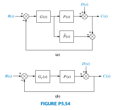
Parabolic trough collector. Effective controller design for parabolic trough collector setups is an active area of research. One of the techniques used for controller design (Camacho, 2012) is Internal Model Control (IMC). Although complete details of IMC will not be presented here, Figure P5.54 (a) shows a block diagram for the IMC setup. Use of IMC assumes a very good knowledge of the plant dynamics. In Figure P5.54(a), the actual plant is P(s). $\tilde{P}\left(s\right)$ is a software model that mimics the plant functions. G(s) is the controller to be designed. It is also assumed that all blocks represent linear time-invariant systems and thus the superposition theorem applies to the system.
a. Use superposition (by assuming D(s) = 0) and Mason's gain formula to find the transfer function $\frac{C\left(s\right)}{R\left(s\right)}$ from command input to system output.

b. Use superposition (by assuming R(s) = 0) and Mason's gain formula to find the transfer function
$\frac{C\left(s\right)}{D\left(s\right)}$ from disturbance input to system output.

c. Use the results of Parts a and b to find the combined output C(s) due to both system inputs.
d. Show that the system of Figure P5.54(a) has the same transfer function as the system in
Figure P5.54(b) when $G_C\left(s\right)=\frac{G\left(s\right)}{1-G\left(s\right)\tilde{P}\left(s\right)}$ .