
Videos
a.
Draw a
a.
Answer to Problem 18CRE
The scatterplot for the data is obtained as follows:
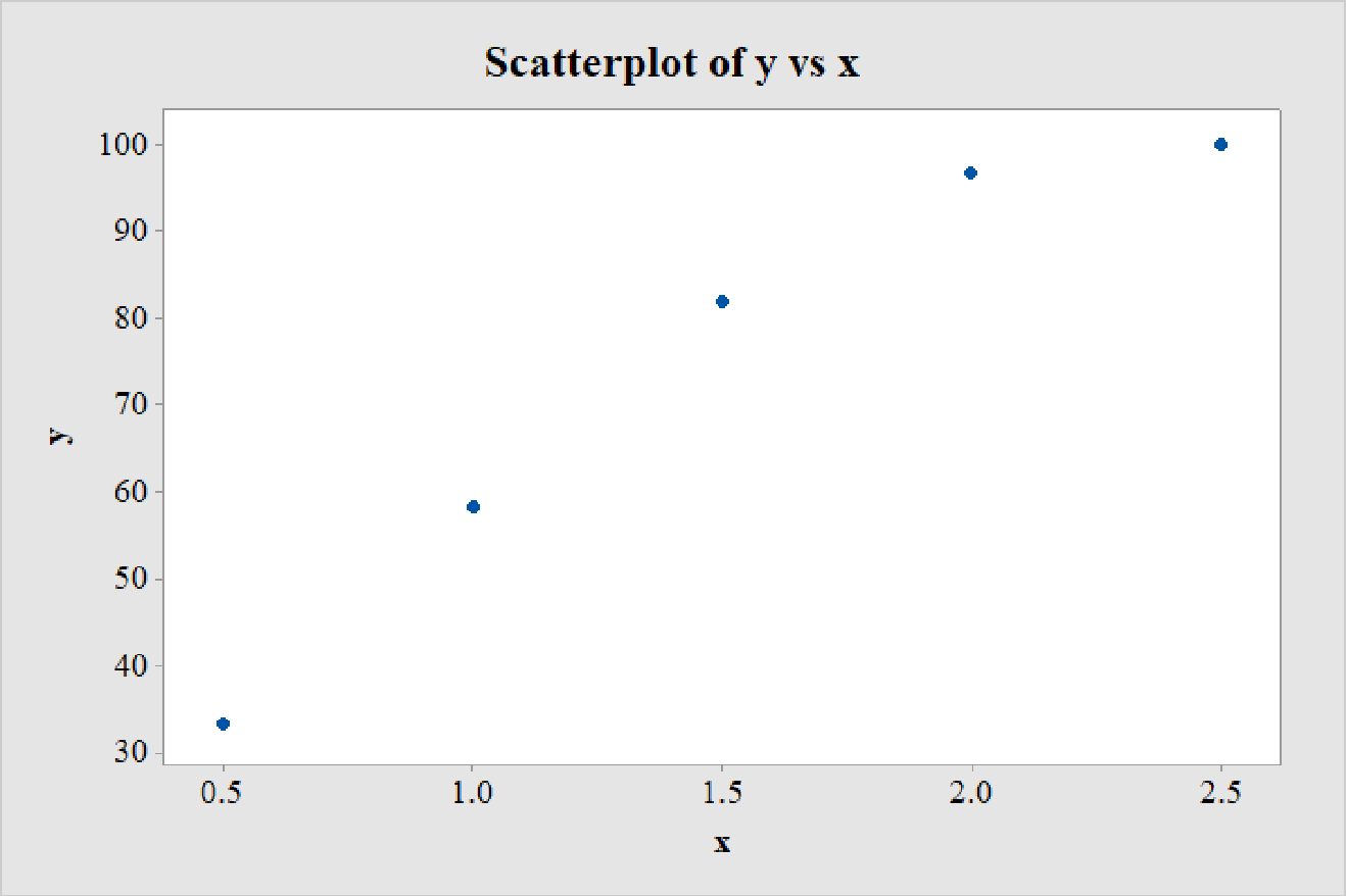
The relationship between the variables is nonlinear.
Explanation of Solution
Calculation:
The data on success (%), y and energy of shock, x is given.
Scatterplot:
Software procedure:
Step-by-step procedure to draw the scatterplot using MINITAB software is given below:
- Choose Graph > Scatterplot.
- Choose Simple, and then click OK.
- Enter the column of y under Y variables.
- Enter the column of x under X variables.
- Click OK.
Thus, the scatterplot is obtained.
A careful observation of the scatterplot reveals that for lower values of x, the points are close to being linear. However, the curvature in the distribution of the points gradually increases with increasing values of x.
Thus, the relationship between the variables is nonlinear.
b.
Fit a least-squares regression line to the data.
Construct a residual plot for the model.
Explain whether the residual plot supports the conclusion in Part a.
b.
Answer to Problem 18CRE
The least-squares regression line for the data is
Explanation of Solution
Calculation:
The least-squares regression line can be obtained using software.
Regression:
Software procedure:
Step by step procedure to get regression equation using MINITAB software is given as,
- Choose Stat > Regression > Regression > Fit Regression Model.
- Under Responses, enter the column of y.
- Under Continuous predictors, enter the columns of x.
- Choose Results and select Analysis of Variance, Model Summary, Coefficients, Regression Equation.
- Choose Graphs, under Residual versus the variables, enter x.
- Click OK on all dialogue boxes.
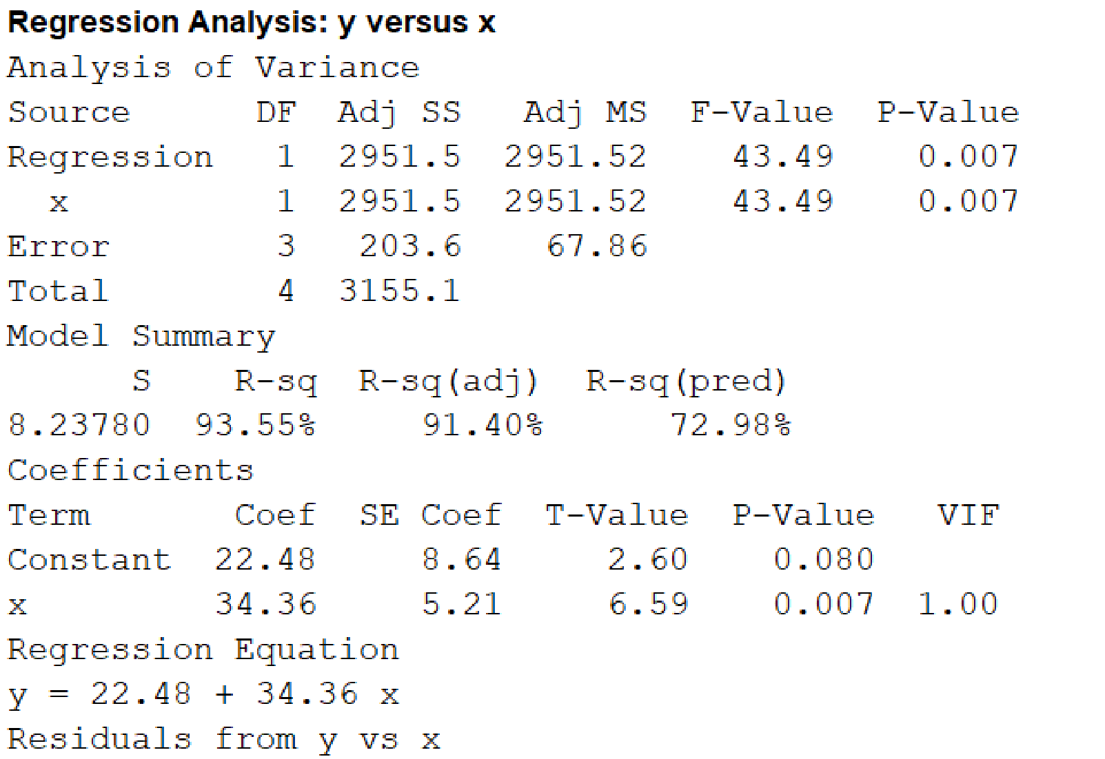
The outputs using MINITAB software is given as follows:
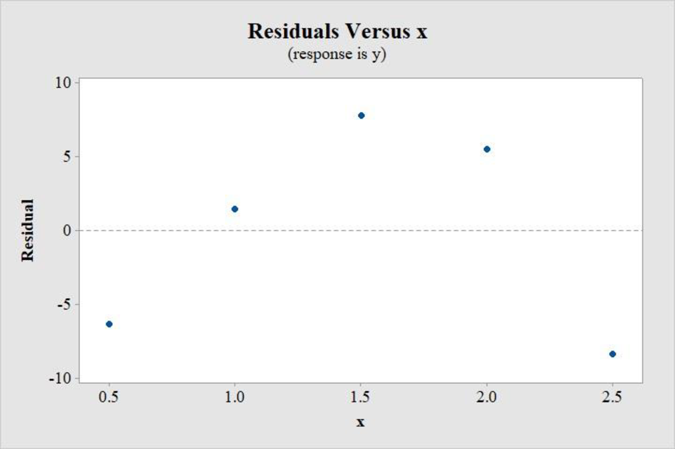
Residual plot:
From the output, the least-squares regression line is:
The ideal residual plot for a linear regression model must not show any pattern and must be randomly distributed. However, this residual plot clearly shows a curved pattern, with an approximate inverted U-shape. This suggests that the data is not linearly distributed.
Thus, the residual plot supports the conclusion in Part a.
c.
Justify whether the transformation
c.
Answer to Problem 18CRE
The transformation
Explanation of Solution
Calculation:
The suitable transformation can be identified by constructing scatterplot between y and
Consider the transformed variable,
Data transformation
Software procedure:
Step-by-step procedure to transform the data using MINITAB software is given below:
- Choose Calc > Calculator.
- Enter the column of sqrt(x) under Store result in variable.
- Enter the formula SQRT(‘x’) under Expression.
- Click OK.
The transformed variable is stored in the column sqrt(x).
Scatterplot:
Software procedure:
Step-by-step procedure to draw the scatterplot using MINITAB software is given below:
- Choose Graph > Scatterplot.
- Choose Simple, and then click OK.
- Enter the column of y under Y variables.
- Enter the column of sqrt(x) under X variables.
- Click OK.
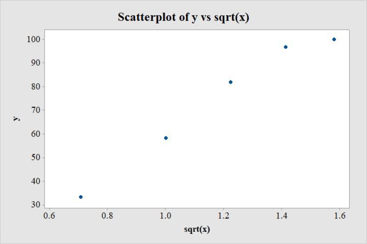
The output obtained using MINITAB is as follows:
Consider the transformed variable,
Data transformation
Software procedure:
Step-by-step procedure to transform the data using MINITAB software is given below:
- Choose Calc > Calculator.
- Enter the column of sqrt(x) under Store result in variable.
- Enter the formula LOGTEN(‘x’) under Expression.
- Click OK.
The transformed variable is stored in the column log(x).
Scatterplot:
Software procedure:
Step-by-step procedure to draw the scatterplot using MINITAB software is given below:
- Choose Graph > Scatterplot.
- Choose Simple, and then click OK.
- Enter the column of y under Y variables.
- Enter the column of log(x) under X variables.
- Click OK.
The output obtained using MINITAB is as follows:
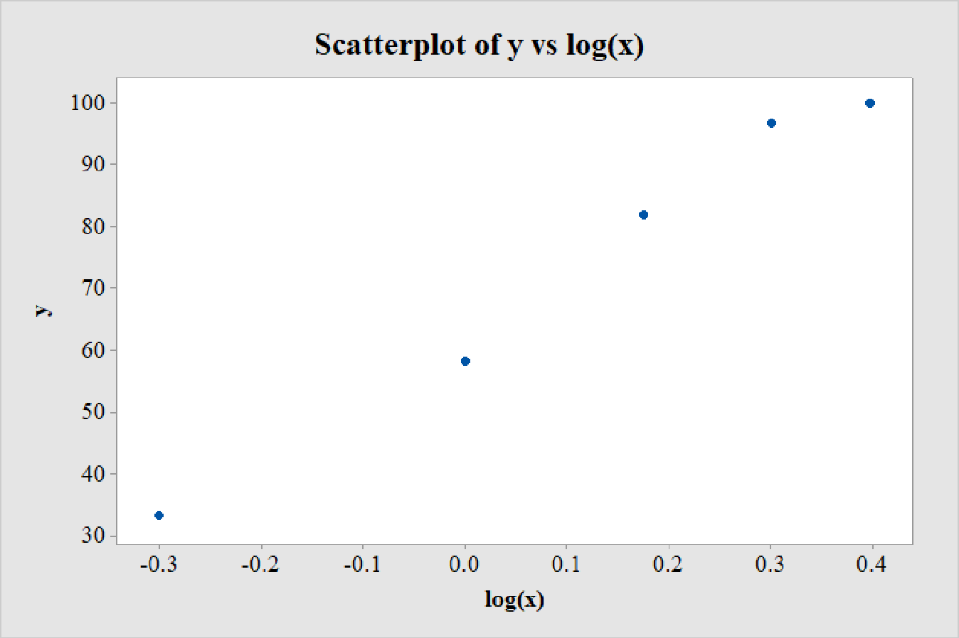
A careful observation of the scatterplot between y and
On the other hand, the scatterplot between y and
Thus, the transformation
d.
Find the least-squares regression line between y and the transformation recommended in the previous part.
d.
Answer to Problem 18CRE
The least-squares regression equation between y and the transformation recommended in the previous part, that is,
Explanation of Solution
Calculation:
The least-squares regression line can be obtained using software.
Regression:
Software procedure:
Step by step procedure to get regression equation using MINITAB software is given as,
- Choose Stat > Regression > Regression > Fit Regression Model.
- Under Responses, enter the column of y.
- Under Continuous predictors, enter the columns of log(x).
- Choose Results and select Analysis of Variance, Model Summary, Coefficients, Regression Equation.
- Click OK on all dialogue boxes.
The outputs using MINITAB software is given as follows:
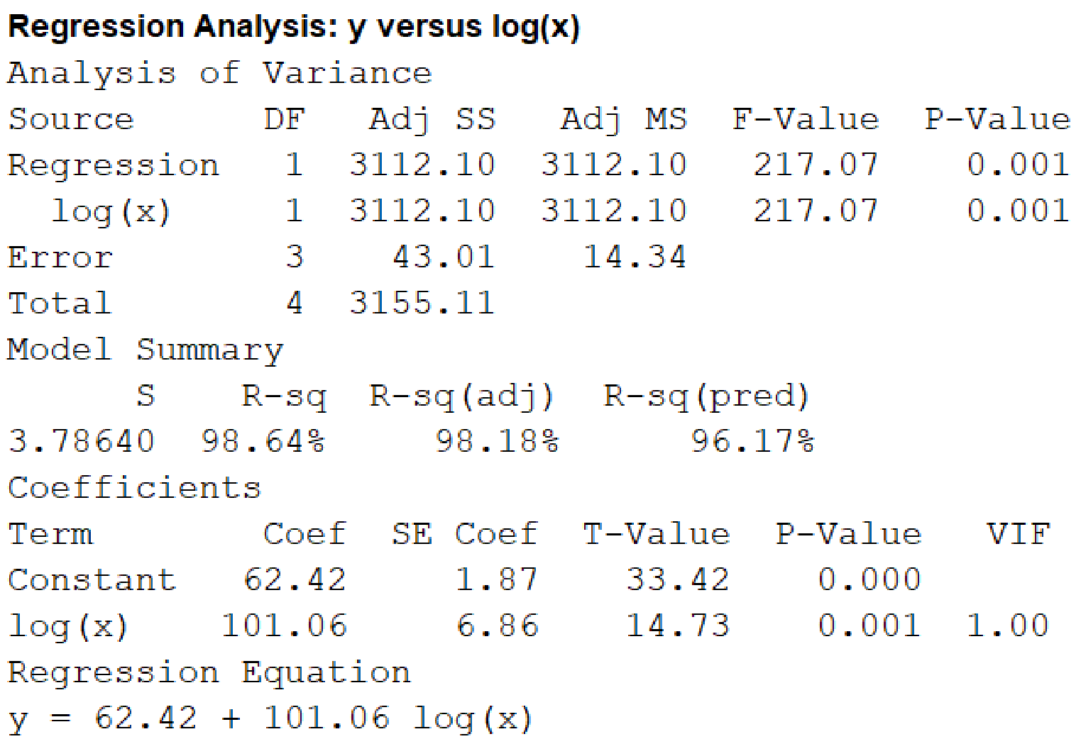
From the output, the least-squares regression equation between y and the transformation recommended in the previous part, that is,
e.
Predict the success for an energy shock 1.75 times the threshold.
Predict the success for an energy shock 0.8 times the threshold.
e.
Answer to Problem 18CRE
The success for an energy shock 1.75 times the threshold is 86.98%.
The success for an energy shock 0.8 times the threshold is 52.63%.
Explanation of Solution
Calculation:
The energy of shock is given as a multiple of the threshold of defibrillation.
For an energy shock 1.75 times the threshold,
Thus, the success for an energy shock 1.75 times the threshold is 86.98%.
For an energy shock 0.8 times the threshold,
Thus, the success for an energy shock 0.8 times the threshold is 52.63%.
Want to see more full solutions like this?
Chapter 5 Solutions
Bundle: Introduction to Statistics and Data Analysis, 5th + WebAssign Printed Access Card: Peck/Olsen/Devore. 5th Edition, Single-Term


- Hoaglin, Mosteller, and Tukey (1983) presented data on blood levels of beta-endorphin as a function of stress. They took beta-endorphin levels for 19 patients 12 hours before surgery and again 10 minutes before surgery. The data are presented below, in fmol/ml Based on these data, what effect does increased stressed have on endorphin levels. include: the hypotheses tested (H0 and H1), the test-statistic and its df, the p-value of the test, and the conclusion as it relates to the research question. Participant 12 hours before 10 minutes before 1 10 6.5 2 6.5 14.0 3 8.0 13.5 4 12 18 5 5.0 14.5 6 11.5…arrow_forwardIn an article in IEEE Transactions on Instrumentation and Measurement (2001, Vol. 50, pp. 986-990), researchers reported on a study of the effects of reducing current draw in a magnetic core by electronic means. They measured the current in a magnetic winding with and without the electronics in a paired experiment. Data for the case without electronics are provided in the Table. Current Without Electronics (mA) Supply Voltage 0.66 7.32 1.32 12.22 1.98 16.34 2.64 23.66 3.3 28.06 3.96 33.39 4.62 34.12 3.28 39.21 5.94 44.21 6.6 47.48 (a) Estimate the correlation coefficient. (b) Test the hypothesis that p = 0 against the alternative p=0 with a = 0.05. What is the P-value? (c) Compute a 95% confidence interval for the correlation coefficient.arrow_forwardHealth care workers who use latex gloves with glove powder on a daily basis are particularly susceptible to developing a latex allergy. Each in a sample of 45 hospital employees who were diagnosed with a latex allergy based on a skin-prick test reported on their exposure to latex gloves. Summary statistics for the number of latex gloves used per week are x = 19.5 and s = 12.1. Complete parts (a) - (d). a. Give a point estimate for the average number of latex gloves used per week by all health care workers with a latex allergy. 19.5 b. Form a 95% confidence interval for the average number of latex gloves used per week by all health care workers with a latex allergy. (Use integers or decimals for any numbers in the expression. Round to two decimal places as needed.)arrow_forward
- Health care workers who use latex gloves with glove powder on a daily basis are particularly susceptible to developing a latex allergy. Each in a sample of 47 hospital employees who were diagnosed with a latex allergy based on a skin-prick test reported on their exposure to latex gloves. Summary statistics for the number of latex gloves used per week are x = 19.3 and s = 12.3. Complete parts (a) - (d). a. Give a point estimate for the average number of latex gloves used per week by all health care workers with a latex allergy. b. Form a 95% confidence interval for the average number of latex gloves used per week by all health care workers with a latex allergy. (Use integers or decimals for any numbers in the expression. Round to two decimal places as needed.) с. Gi a practical interpretation of the interval, part (b). A. One can be 95% confident that latex gloves cause allergies for all who use a number of gloves contained in the interval. B. One can be 95% confident that the average…arrow_forwardHealth care workers who use latex gloves with glove powder on a daily basis are particularly susceptible to developing a latex allergy. Each in a sample of 44 hospital employees who were diagnosed with a latex allergy based on a skin-prick test reported on their exposure to latex gloves. Summary statistics for the number of latex gloves used per week are x= 19.4 and s = 11.7. Complete parts (a) - (d). a. Give a point estimate for the average number of latex gloves used per week by all health care workers with a latex allergy. b. Form a 95% confidence interval for the average number of latex gloves used per week by all health care workers with a latex allergy. (Use integers or decimals for any numbers in the expression. Round to two decimal places as needed.) c. Give a practical interpretation of the interval, part (b). O A. One can be 95% confident that latex gloves cause allergies for all who use a number of gloves contained in the interval. O B. One can be 95% confident that the…arrow_forwardAn article in the Journal of Environmental Engineering (1989, Vol. 115(3), pp. 608–619) reported the results of a study on the occurrence of sodium and chloride in surface streams in central Rhode Island. The following data are chloride concentration y (in milligrams per liter) and roadway area in the watershed x (in percentage).arrow_forward
- The spotted lanternfly, Lycorma delicatula, is an invasive species to the United States that has the potential to do significant agricultural damage. An ecologist is studying the relationship between the size of the female spotted lanternflies and the number of eggs they produce. The data are summarized below. Length of insect: AVG = 1 inch, SD = 0.15 inchNumber of eggs: AVG = 40 eggs, SD = 5 eggsr = 0.2 Using regression, we can say that the average number of eggs produced by female spotted lanternflies who are 1.1 inch long is closest to... Group of answer choices 42 39 40 41arrow_forwardAn article in Technometrics (1974, Vol. 16, pp. 523–531) considered the following stack-loss data from a plant oxidizing ammonia to nitric acid. Twenty-one daily responses of stack loss (the amount of ammonia escaping) were measured with air flow x1, temperature x2, and acid concentration x3. y = 42, 37, 37, 28, 18, 18, 19, 20, 15, 14, 14, 13, 11, 12, 8, 7, 8, 8, 9, 15, 15 x1 = 80, 80, 75, 62, 62, 62, 62, 62, 58, 58, 58, 58, 58, 58, 50, 50, 50, 50, 50, 56, 70 x2 = 27, 27, 25, 24, 22, 23, 24, 24, 23, 18, 18, 17, 18, 19, 18, 18, 19, 19, 20, 20, 20 x3 = 89, 88, 90, 87, 87, 87, 93, 93, 87, 80, 89, 88, 82, 93, 89, 86, 72, 79, 80, 82, 91 (a) Fit a linear regression model relating the results of the stack loss to the three regressor variables. (b) Estimate σ2. (c) Find the standard error se(βj). (d) Use the model in part (a) to predict stack loss when x1 = 60, x2 = 26, and x3 = 85.arrow_forwardThe article in the ASCE Journal of Energy Engineering (1999, Vol. 125, pp.59-75) describes a study of the thermal inertia properties of autoclaved aerated concrete used as a building material. Five samples of the material were tested in a structure, and the average interior temperatures (°C) reported were as follows: 23.01, 22.22, 22.04, 22.62, and 22.59. Test that the average interior temperature is equal to 22.5°C using alpha (a) = 0.05. This problem is a test on what population parameter? What is the null and alternative hypothesis? What are the Significance level and type of test? What standardized test statistic will be used? What is the standard test statistic? What is the Statistical Decision? What is the statistical decision in the statement form?arrow_forward
- Solve An article in the ASCE Journal of Energy Engineering (1999, Vol. 125, pp.59-75) describes a study of the thermal inertia properties of autoclaved aerated concrete used as a building material. Five samples of the material were tested in a structure, and the average interior temperatures (°C) reported were as follows: 23.01, 22.22, 22.04, 22.62, and 22.59. Test that the average interior temperature is equal to 22.5°C using alpha (a) = 0.05. 1.)This problem is a test on what population parameter? a.Variance/ Standard Deviation b.Mean c.Population Proportion d.None of the above 2.)What is the null and alternative 3 points hypothesis? a.Ho / (theta = 22.5) , Ha: (0 # 22.5) b.Ho / (theta > 22.5) , Ha: (0 # 22.5) c.Ho / (theta < 22.5) , Ha: (theta >= 22.5) d.None of the above 3.)What are the Significance level 3 points and type of test? alpha = 0.05 two-tailed alpha = 0.95 two-tailed alpha = 0.95 one-tailed None of the above 4.)What standardized test statistic will…arrow_forwardAn article in Journal of Food Science [“Prevention of Potato Spoilage During Storage by Chlorine Dioxide” (2001, Vol. 66(3), pp. 472–477)] reported on a study of potato spoilage based on different conditions of acidified oxine (AO), which is a mixture of chlorite and chlorine dioxide. The data follow: ∑X1i=230, ∑X21i=17200, n1=3. ∑X2i=150, ∑X22i=8100, n2=3. ∑X3i=60, ∑X23i=4500, n3=3. ∑X4i=65, ∑X24i=1625, n4=3. where group 1 has AO = 50ppm, group 2 has AO = 100ppm, group 3 has AO = 200ppm, group 4 has AO = 400ppm. Complete the ANOVA table below Source df sum of square mean square F p-value Between Within N/A N/A Total 11 N/A N/A N/A At α=0.05, do we reject the null hypothesis that AO does not affect spoilage?arrow_forwardAn article in the ACI Materials Journal (Vol. 84, 1987, pp. 213-216) describes several experiments investigating the rodding of concrete to remove trapped air. A 3-inch x 6-inch cylinder was used, and the number of times this rod was used is the design variable. The resulting compressive strength of the concrete specimen is the response. The data are shown in the following table. Compressive Strength (psi) Rodding Level Observations 10 1530 1530 1440 15 1610 1650 1500 20 1560 1730 1530 25 1500 1490 1510 Calculate the test statistic fo- Input answer up to 2 decimal places. Test Statisticf = Blank 1arrow_forward
 Calculus For The Life SciencesCalculusISBN:9780321964038Author:GREENWELL, Raymond N., RITCHEY, Nathan P., Lial, Margaret L.Publisher:Pearson Addison Wesley,
 Glencoe Algebra 1, Student Edition, 9780079039897...AlgebraISBN:9780079039897Author:CarterPublisher:McGraw Hill