
Concept explainers
Videos
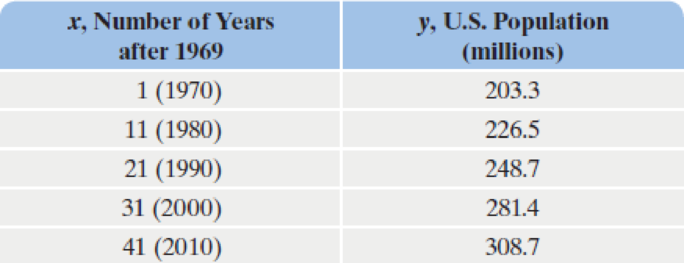
In Example 1 on page 520, we used two data points and an exponential function to model the population of the United States from 1970 through 2010. The data are shown again in the table. Use all five data points to solve Exercises 66–70.
66.
- a. Use your graphing utility’s exponential regression option to obtain a model of the form y = abx that fits the data. How well does the
correlation coefficient , r, indicate that the model fits the data? - b. Rewrite the model in terms of base e. By what percentage is the population of the United States increasing each year?
67. Use your graphing utility’s logarithmic regression option to obtain a model of the form y = a + b ln x that fits the data. How well does the correlation coefficient, r, indicate that the model fits the data?
68. Use your graphing utility’s linear regression option to obtain a model of the form y = ax + b that fits the data. How well does the correlation coefficient, r, indicate that the model fits the data?
69. Use your graphing utility’s power regression option to obtain a model of the form y = axb that fits the data. How well does the correlation coefficient, r, indicate that the model fits the data?
70. Use the values of r in Exercises 66–69 to select the two models of best fit. Use each of these models to predict by which year the U.S. population will reach 335 million. How do these answers compare to the year we found in Example 1, namely 2020? If you obtained different years, how do you account for this difference?
Want to see the full answer?
Check out a sample textbook solution
Chapter 4 Solutions
College Algebra Essentials


- In Exercises 1–6, solve for x.arrow_forwardIn Exercises 13–24, draw a dependency diagram and write a Chain Rule formula for each derivative.arrow_forwardThe Internal Revenue Service Restructuring and Reform Act (RRA) was signed into law by President Bill Clinton in 1998. A major objective of the RRA was to promote electronic filing of tax returns. The data in the table that follows show the percentage of individual income tax returns filed electronically for filing years 2000–2008. Since the percentage P of returns filed electronically depends on the filing year y and each input corresponds to exactly one output, the percentage of returns filed electronically is a function of the filing year;so P(y) represents the percentage of returns filed electronically for filing year y. (a) Find the average rate of change of the percentage of e-filed returns from 2000 to 2002. (b) Find the average rate of change of the percentage of e-filed returns from 2004 to 2006. (c) Find the average rate of change of the percentage of e-filed returns from 2006 to 2008. (d) What is happening to the average rate of change as time passes?arrow_forward
- Exercises 93–94: Energy The following graph shows U.S. Energy consumption. 400 350 300 250 200 150 100 50 04 1970 1990 2010 Year 93. When was energy consumption increasing? 94. When was energy consumption decreasing? Energy (millions of Btu)arrow_forwardRegression and Predictions. Exercises 13–28 use the same data sets as Exercises 13–28 in Section 10-1. In each case, find the regression equation, letting the first variable be the predictor (x) variable. Find the indicated predicted value by following the prediction procedure summarized in Figure 10-5 on page 493. Old Faithful Using the listed duration and interval after times, find the best predicted “interval after” time for an eruption with a duration of 253 seconds. How does it compare to an actual eruption with a duration of 253 seconds and an interval after time of 83 minutes?arrow_forwardNational Debt The size of the total debt owed by the UnitedStates federal government continues to grow. In fact,according to the Department of the Treasury, the debt perperson living in the United States is approximately $53,000(or over $140,000 per U.S. household). The following datarepresent the U.S. debt for the years 2001–2014. Since thedebt D depends on the year y, and each input correspondsto exactly one output, the debt is a function of the year. SoD1y2 represents the debt for each year y. Source: www.treasurydirect.govDebt (billions Debt (billionsYear of dollars) Year of dollars)2001 5807 2008 10,0252002 6228 2009 11,9102003 6783 2010 13,5622004 7379 2011 14,7902005 7933 2012 16,0662006 8507 2013 16,7382007 9008 2014 17,824 (a) Plot the points 12001, 58072, 12002, 62282, and so on ina Cartesian plane.(b) Draw a line segment from the point 12001, 58072 to12006, 85072. What does the slope of this line segmentrepresent?(c) Find the average rate of change of the debt from 2002…arrow_forward
- Q. Table provided gives data on gross domestic product (GDP) for the United States for the years 1959–2005. a. Plot the GDP data in current and constant (i.e., 2000) dollars against time. b. Letting Y denote GDP and X time (measured chronologically starting with 1 for 1959, 2 for 1960, through 47 for 2005), see if the following model fits the GDP data: Yt = β1 + β2 Xt + ut Estimate this model for both current and constant-dollar GDP. c. How would you interpret β2? d. If there is a difference between β2 estimated for current-dollar GDP and that estimated for constant-dollar GDP, what explains the difference? e. From your results what can you say about the nature of inflation in the United States over the sample period?arrow_forwardproblen 1.4arrow_forwardWorld Military Expenditure The following chart shows total military and arms trade expenditure from 2011–2020 (t = 1 represents 2011). †A bar graph titled "World military expenditure" has a horizontal t-axis labeled "Year since 2010" and a vertical axis labeled "$ (billions)". The bar graph has 10 bars. Each bar is associated with a label and an approximate value as listed below. 1: 1,800 billion dollars 2: 1,775 billion dollars 3: 1,750 billion dollars 4: 1,730 billion dollars 5: 1,760 billion dollars 6: 1,760 billion dollars 7: 1,850 billion dollars 8: 1,900 billion dollars 9: 1,950 billion dollars 10: 1,980 billion dollars (a) If you want to model the expenditure figures with a function of the form f(t) = at2 + bt + c, would you expect the coefficient a to be positive or negative? Why? HINT [See "Features of a Parabola" in this section.] We would expect the coefficient to be positive because the curve is concave up. We would expect the coefficient to be negative because the…arrow_forward
- Sec3.4#55arrow_forwardInsurance Rates The following table gives themonthly insurance rates for a $100,000 life insurancepolicy for smokers 35–50 years of age.a. Create a scatter plot for the data.b. Does it appear that a quadratic function can beused to model the data? If so, find the best-fittingquadratic model.c. Find the power model that is the best fit for the data.d. Compare the two models by graphing each modelon the same axes with the data points. Whichmodel appears to be the better fit?arrow_forwardFor Exercises 33–38, find the exact value of each expression without the use of a calculator. (See Example 5)arrow_forward
 Algebra & Trigonometry with Analytic GeometryAlgebraISBN:9781133382119Author:SwokowskiPublisher:Cengage