
(a)
Estimated regression line.
(a)
Explanation of Solution
The formula for the regression equation is:
Run the ordinary least squares method for the given data in excel. The results drawn are as follows:
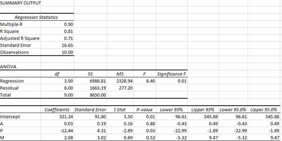
Use the summary output to find the estimated regression equation as follows:
(b)
The economic interpretation of the estimated intercept (a) and slope (b) coefficients.
(b)
Explanation of Solution
Interpretation of estimated intercept (a) coefficient:
When the selling
Interpretation of estimated slope (b) coefficient:
For a given level of selling price and disposable income, an additional $1,000 promotional expenditures lead to a rise in sales by 0.03×1000 = 30 gallons on average.
For a given level of promotional expenditure and selling price, an additional $1,000 disposable income leads to a rise in sales by 2.08×1000 = 2,080 gallons on an average.
For a given level of promotional expenditure and disposable income, an additional $1/gallon lead to falling in sales by 12.44×1000 = 12,440 gallons on an average.
(c)
The hypothesis that there is no relationship between the variables at 0.05 significance level.
(c)
Explanation of Solution
Conduct the t-test to know the statistical significance of the independent variables A, Pand M. The test statistic can be calculated using the following formula:
The t-statistic follows t-distribution with n-1 degrees of freedom.
For variable A, t-test is conducted as follows:
According to the summary output, the t-statistic for A variable is equal to 0.16.
At 5% significance level and 10-1=9 degrees of freedom, the critical value is equal to 2.262.
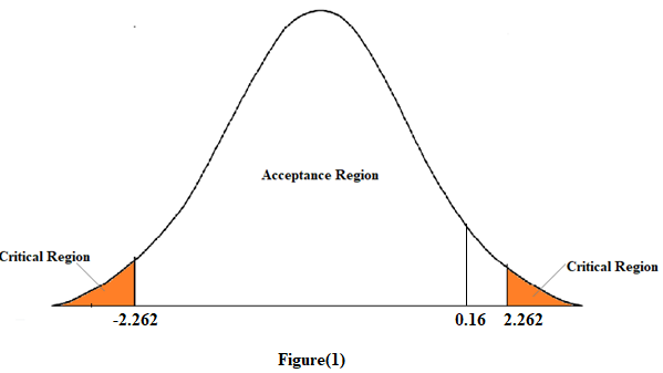
In figure (1), since the calculated t-statistic lies in the acceptance region. Therefore, we accept the null hypothesis. This means that the variable A is not statistically significant.
For variable P, t-test is conducted as follows:
According to the summary output, the t-statistic for P variable is equal to -2.89. At 5% significance level and 10-1=9 degrees of freedom, the critical value is equal to 2.262.
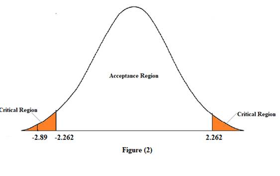
In figure (2), since the calculated t-statistic lies in the critical region. Therefore, we reject the null hypothesis. This means that the variable Pis statistically significant.
For variable M, t-test is conducted as follows:
According to the summary output, the t-statistic for M variable is equal to 0.69.
At 5% significance level and 10-1=9 degrees of freedom, the critical value is equal to 2.262.
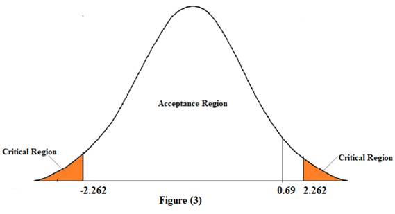
In figure (3), since the calculated t-statistic lies in the acceptance region. Therefore, we accept the null hypothesis. This means that the M variable is not statistically significant.
(d)
Coefficient of determination.
(d)
Explanation of Solution
The coefficient of determination measures the proportion of variance predicted by the independent variable in the dependent variable. It is denoted as R2.
According to the summary output, the value of R2 is equal to 0.81. This means that the regression equation predicts 81% of the variance in sales.
(e)
(e)
Explanation of Solution
The value of F-statistic is given as 8.40. And the critical value at 0.05 significance level is equal to 0.01.
Since F-statistic is greater than the critical value, thus, the overall model is statistically significant.
(f)
Best estimate of the product sales when the selling price is $14.50. And an approximate 95 percent prediction interval.
(f)
Explanation of Solution
According to the regression statistics of the summary output, for a given level of promotional expenditure and disposable income, $14.50/gallon lead to fall in sales by 12.44×14.50×1000 = 180,380 gallons on an average.
According to the regression statistics in the summary output, a 95% confidence interval for the P variable ranges from -22.99 to -1.89.
(g)
(g)
Explanation of Solution
Formula to calculate elasticity in linear regression model is as follows:
At given value of P variable equal to 14.50, the estimated value of Y variable is equal to 180,380.
Thus, price
Thus, the price elasticity of demand at a selling price of $14.50 is equal to -0.001.
Want to see more full solutions like this?
Chapter 4 Solutions
Bundle: Managerial Economics: Applications, Strategies And Tactics, 14th + Mindtap Economics, 1 Term (6 Months) Printed Access Card

- not use ai pleasearrow_forward• Prismatic Cards: A prismatic card will be a card that counts as having every suit. We will denote, e.g., a prismatic Queen card by Q*. With this notation, 2.3045 Q would be a double flush since every card is a diamond and a heart. • Wild Cards: A wild card counts as having every suit and every denomination. Denote wild cards with a W; if there are multiple, we will denote them W₁, W2, etc. With this notation, W2 20.30054 would be both a three-of-a-kind (three 2's) and a flush (5 diamonds). If we add multiple wild cards to the deck, they count as distinct cards, so that (e.g.) the following two hands count as "different hands" when counting: W15 5Q and W255◊♡♡♣♣ In addition, 1. Let's start with the unmodified double-suited deck. (a) Call a hand a flush house if it is a flush and a full house, i.e. if all cards share a suit and there are 3 cards of one denomination and two of another. For example, 550. house. How many different flush house hands are there? 2. Suppose we add one wild…arrow_forwardnot use ai pleasearrow_forward
- In a classic oil-drilling example, you are trying to decide whether to drill for oil on a field that might or might not contain any oil. Before making this decision, you have the option of hiring a geologist to perform some seismic tests and then predict whether there is any oil or not. You assess that if there is actually oil, the geologist will predict there is oil with probability 0.85 . You also assess that if there is no oil, the geologist will predict there is no oil with probability 0.90. Please answer the two questions below, as I am trying to ensure that I am correct. 1. Why will these two probabilities not appear on the decision tree? 2. Which probabilities will be on the decision tree?arrow_forwardAsap pleasearrow_forwardnot use ai pleasearrow_forward
- not use ai pleasearrow_forwardIn this question, you will test relative purchasing parity (PPP) using the data. Use yearly data from FRED website from 1971 to 2020: (i) The Canadian Dollars to U.S. Dollar Spot Exchange Rate (ER) (ii) Consumer price index for Canada (CAN_CPI), and (iii) Consumer price index for the US (US_CPI). Inflation is measured by the consumer price index (CPI). The relative PPP equation is: AE CAN$/US$ ECAN$/US$ = π CAN - πUS Submit the Excel sheet that you worked on. 1. First, compute the percentage change in the exchange rate (left-hand side of the equation). Caculate the variable for each year from 1972 to 2020 in Column E (named Change_ER) of the Excel sheet. For example, for 1972, compute E3: (B3-B2)/B2). ER1972 ER1971 ER 1971 (in Excel, the formula in cellarrow_forwardnot use ai pleasearrow_forward
- 8. The current price of 3M stock is $87 per share. The previous dividend paid was $5.96, and the next dividend is $6.25, assuming a growth rate of 4.86% per year. What is the forward (next 12 months) dividend yield? Show at least two decimal places, as in x.xx% %arrow_forwardJoy's Frozen Yogurt shops have enjoyed rapid growth in northeastern states in recent years. From the analysis of Joy's various outlets, it was found that the demand curve follows this pattern: Q=200-300P+1201 +657-250A +400A; where Q = number of cups served per week P = average price paid for each cup I = per capita income in the given market (thousands) Taverage outdoor temperature A competition's monthly advertising expenditures (thousands) = A; = Joy's own monthly advertising expenditures (thousands) One of the outlets has the following conditions: P = 1.50, I = 10, T = 60, A₁ = 15, A; = 10 1. Estimate the number of cups served per week by this outlet. Also determine the outlet's demand curve. 2. What would be the effect of a $5,000 increase in the competitor's advertising expenditure? Illustrate the effect on the outlet's demand curve. 3. What would Joy's advertising expenditure have to be to counteract this effect?arrow_forwardThe Compute Company store has been selling its special word processing software, Aceword, during the last 10 months. Monthly sales and the price for Aceword are shown in the following table. Also shown are the prices for a competitive software, Goodwrite, and estimates of monthly family income. Calculate the appropriate elasticities, keeping in mind that you can calculate an elasticity measure only when all other factors do not change (using Excel). For example, price elasticities, months 1-2. Month Price Aceword Quantity Aceword Family Income Price Goodwrite 1 $120 200 $4,000 $130 21 120 210 4,000 145 3 120 220 4,200 145 4 110 240 4,200 145 90 5 115 230 4,200 145 6 115 215 4,200 125 10 7899 115 220 4,400 125 105 230 4,400 125 105 235 4,600 125 105 220 4,600 115arrow_forward
 Managerial Economics: Applications, Strategies an...EconomicsISBN:9781305506381Author:James R. McGuigan, R. Charles Moyer, Frederick H.deB. HarrisPublisher:Cengage Learning


