
Concept explainers
Videos
(a)
The random numbers by summing twelve uniform variables and subtracting 6.
(a)
Answer to Problem 87E
Solution: The simulated distribution is shown in the below table.
| 0.543534 | ||||
| 0.248992 | 1.493676 | 1.535747 | ||
| 0.742845 | 0.170866 | 0.394907 | 0.799959 | 2.122601 |
| 0.264532 | 1.407664 | 1.283963 | ||
| 0.442991 | 0.720228 | 2.229499 | 1.609478 | |
| 0.708811 | 0.534153 | 0.903971 | 0.06244 | |
| 1.238842 | 0.142653 | 0.134968 | ||
| 0.387513 | 0.525326 | 1.013777 | 0.665731 | |
| 2.04422 | ||||
| 0.415165 | 0.098935 | 2.275969 | 0.559715 | 0.925708 |
| 1.306352 | ||||
| 0.199455 | 0.606878 | 2.31169 | 1.041178 | |
| 1.371048 | 0.882886 | 0.45936 | 0.613565 | |
| 1.145033 | 1.460973 | |||
| 1.84498 | 1.512605 | 0.462096 | ||
| 1.207655 | 0.98702 | 0.661045 | 1.011263 | 0.805521 |
| 0.129918 | 0.287478 | 0.574382 | ||
| 0.203774 | 0.378354 | 1.203827 | ||
| 0.500351 | 1.292136 | 0.606476 | ||
| 1.330552 | 0.166358 |
Explanation of Solution
The below steps are followed in Minitab software to obtain the distribution for the variable.
Step 1: Open the Minitab worksheet. Go to Calc > Random Data> Uniform.
Step 2: Input 100 as the number of rows of data. Input C1-C12 in the “Store in column(s)” option and specify the Lower endpoint and the Upper endpoint as 0 and 1 respectively.
Step 3: Click OK.
Step 4: Go to Calc > Calculator.
Step 5: Enter C13 in “Store result in variable” and in “Expression”, write the expression as
Step 6: Click OK.
The generated random number is shown in the below table.
| 0.543534 | ||||
| 0.248992 | 1.493676 | 1.535747 | ||
| 0.742845 | 0.170866 | 0.394907 | 0.799959 | 2.122601 |
| 0.264532 | 1.407664 | 1.283963 | ||
| 0.442991 | 0.720228 | 2.229499 | 1.609478 | |
| 0.708811 | 0.534153 | 0.903971 | 0.06244 | |
| 1.238842 | 0.142653 | 0.134968 | ||
| 0.387513 | 0.525326 | 1.013777 | 0.665731 | |
| 2.04422 | ||||
| 0.415165 | 0.098935 | 2.275969 | 0.559715 | 0.925708 |
| 1.306352 | ||||
| 0.199455 | 0.606878 | 2.31169 | 1.041178 | |
| 1.371048 | 0.882886 | 0.45936 | 0.613565 | |
| 1.145033 | 1.460973 | |||
| 1.84498 | 1.512605 | 0.462096 | ||
| 1.207655 | 0.98702 | 0.661045 | 1.011263 | 0.805521 |
| 0.129918 | 0.287478 | 0.574382 | ||
| 0.203774 | 0.378354 | 1.203827 | ||
| 0.500351 | 1.292136 | 0.606476 | ||
| 1.330552 | 0.166358 |
(b)
To find: The numerical and graphical summary of the obtained distribution.
(b)
Answer to Problem 87E
Solution: The shape of the distribution is more or less symmetric and the centre of the curve is near the
Explanation of Solution
Calculation: To obtain the numerical summary of the data, the below steps are followed in the Minitab software.
Step 1: Go to Stat
Step 2: Select ‘C13’ in the variable option.
Step 3: Click on the Statistics button.
Step 4:Select minimum, maximum, mean and standard deviation.
Step 5: Click OK.
The mean, standard deviation, minimum, and maximum values are obtained as 0.2460, 0.994,
Graph: The below steps are followed in Minitab software to obtain the histogram for the distribution.
Step 1: Insert all the observations in the worksheet.
Step 2: Go to Graph
Step 3: Select ‘C13’ in the ‘Graph variable’ option.
Step 4: Click OK.
The obtained histogram is,
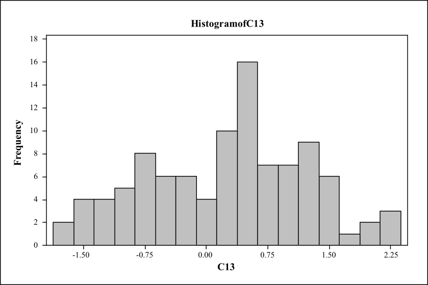
Interpretation: The histogram shows that the shape of the distribution is more or less symmetric. Moreover, the centre of the curve is near the mean value, 0.2460. The standard deviation of the distribution is almost 1. The distribution can be considered as approximately normal.
(c)
The summary of the findings of the provided simulation.
(c)
Answer to Problem 87E
Solution: The simulated distribution is approximated by the standard
Explanation of Solution
The 100 samples are generated by summing 12 uniform variables and subtracting 6 from the sum. The mean of the distribution is 0.2460 and standard deviation is 1. The obtained distribution can be approximated by the standard normal distribution whose mean is 0 and standard deviation is 1.
Want to see more full solutions like this?
Chapter 3 Solutions
EBK INTRODUCTION TO THE PRACTICE OF STA


 Big Ideas Math A Bridge To Success Algebra 1: Stu...AlgebraISBN:9781680331141Author:HOUGHTON MIFFLIN HARCOURTPublisher:Houghton Mifflin Harcourt
 Glencoe Algebra 1, Student Edition, 9780079039897...AlgebraISBN:9780079039897Author:CarterPublisher:McGraw Hill
 Linear Algebra: A Modern IntroductionAlgebraISBN:9781285463247Author:David PoolePublisher:Cengage Learning
 Holt Mcdougal Larson Pre-algebra: Student Edition...AlgebraISBN:9780547587776Author:HOLT MCDOUGALPublisher:HOLT MCDOUGAL