
Concept explainers
Videos
The velocity of water flow through the porous media can be related to head by D'Arcy's law
where K is the hydraulic conductivity and
To calculate: The water flowsvelocity through the porous media for the Prob. 32.8, if the hydraulic conductivity is
Answer to Problem 9P
Solution:
The water flow velocity at every node is,
| -5.205E-04 | -5.542E-04 | -6.593E-04 | -7.249E-04 |
| -5.079E-04 | -5.315E-04 | -6.989E-04 | -7.942E-04 |
| -4.668E-04 | -3.967E-04 | -4.429E-04 |
Explanation of Solution
Given Information:
Write the expression for D’Arcy’s law.
Here,
The hydraulic conductivity is
Formula used:
Consider the Laplace Equation,
Write the central difference approximation for the second derivative.
Calculation:
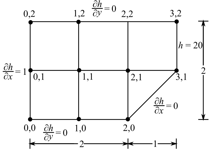
Refer to Figure P32.8, draw the nodal diagram.
Recall the Laplace Equation,
The central difference approximation applies for the second derivative in above Laplace equation,
At the node,
Approximate the all external nodes with a central finite difference,
Thus,
Now with a central finite difference, approximate the external nodes.
Solve further,
Substitute (3) and (4) in (2).
Similarly, at the node,
Similarly, at the node,
Similarly, at the node,
Similarly, at the node,
Similarly, at the node,
Similarly, at the node,
Similarly, at the node,
Similarly, at the node,
Thus, the system of all linear equations is,
And,
And,
Write all equation in matrix form.
Use the MATLAB to solve the above equations, write the following code in MATLAB.
The output is,
Thus, the distribution of head of the system is shown below.
| 16.3372 | 17.37748 | 18.55022 | 20 |
| 16.29691 | 17.31126 | 18.4117 | 20 |
| 16.22792 | 17.15894 | 17.78532 |
Now from the above table find the value of
And
Calculate the value of
And,
Calculate all the value of
| 1.04029 | 1.10651 | 1.31126 | 1.44978 |
| 1.01435 | 1.05740 | 1.34437 | 1.58830 |
| 0.93102 | 0.77870 | 0.62638 |
Calculate the value of
Calculate all the value of
| 0.04029 | 0.06623 | 0.13852 | 0.00000 |
| 0.05464 | 0.10927 | 0.38245 | 0.00000 |
| 0.06898 | 0.15232 | 0.62638 |
Now calculate the value of
Substitute the values of
For
Calculate for every node the value of
| 1.04107 | 1.10849 | 1.31855 | 1.44978 |
| 1.01582 | 1.06303 | 1.39771 | 1.58830 |
| 0.93357 | 0.79345 | 0.88583 |
Apply the D’Arcy law to find the discharge velocity in the n direction:
Here,
Now Calculate for the velocity (
Calculate the velocity for every node same way, and got the following table:
| -5.205E-04 | -5.542E-04 | -6.593E-04 | -7.249E-04 |
| -5.079E-04 | -5.315E-04 | -6.989E-04 | -7.942E-04 |
| -4.668E-04 | -3.967E-04 | -4.429E-04 |
Want to see more full solutions like this?
Chapter 32 Solutions
EBK NUMERICAL METHODS FOR ENGINEERS


- A vertical jet of water thru a nozzle supports a load of 200 N at a constant vertical height of 2m from the tip of the nozzle. The diameter of the jet is 25mm. Find the velocity of the jet at the nozzle tip. A. 28.32 m/sB. 23.28 m/sC. 21.13 m/sD. 22.82 m/sarrow_forward5- Water flows over a flat surface at 4 ft/s, as shown in Fig. 5 . A pump draws off water through a narrow slit at a vol- ume rate of 0.1 ft/s per foot length of the slit. Assume that the fluid is incompressible and inviscid and can be represented by the com- bination of a uniform flow and a sink. Locate the stagnation point on the wall (point A) and determine the equation for the stagnation streamline. How far above the surface, H, must the fluid be so that it does not get sucked into the slit? 4 ft/s 0.1 fts (per foot of length of slit)arrow_forwardA pump draws water from open reservoir A at 20 ft above pump centerline and lifts to an open reservoir B at 280 ft above pump centerline. The loss of head at the suction is 3 times the velocity head at the 6 inches suction pipe and at the discharge is 20 times the velocity head at the 4 inches discharge pipe. The pump discharge is 200 GPM. a. The total dynamic head in ft. 268.32 367.62 288.32 b. The water power in horsepower 31.49 13.54 19.45arrow_forward
- A circular pipe CD carries 1/3rd of flow in AB. Find volume rate of flow in AB, diameter of BC, velocity in CD and diameter of CE. B, 4Q o8 m 4m/s +2.2 m 1.8m/s 2.25m/sarrow_forward1.28. The performance curve for the fan of Problem 1.27 can be approx- imated by a straight line through its BEP (using techniques devel- oped in Chapter 7). The curve is Aps = 4488 – 166Q, with ApT in Pa and Q in m³/s. If this fan is connected to a 1-m dia- meter duct (f = 0.045) whose length is 66 m, what flow rate will result? %3Darrow_forwardA pump impeller rotating at 1400 rpm has an outside radius of 21 cm, the vane outlet angle B2 is 158* and the radial velocity at the outlet Cr2 is 4 m/s. Assuming radial flow at inlet, draw the theoretical outlet velocity diagram and calculate the various velocities and angles. What is the theoretical head Ho, in meters, assuming that the circulatory flow coefficient n = 1. 91.84 65.60 46.86 128.58 180.01 calculate the water horsepower. 52.4 22.1 78.9 16.8 34.8arrow_forward
- 16. Consider the the equation for volumetric flow rate by Bernoulli obstruction theory [2Ap/ By this theory, all else being equal, a doubling of the pressure difference corresponds to increase in flow rate by what factor? Ⓐ: 1:41 B. 2 C. 4 D. 0.707 E. 8.0arrow_forward7) A pump has the following characteristic: Volume flow rate 23 46 69 92 115 (m³/h) Head (m) 17 16 13.5 10.5 6.6 The is used to pump water from a lower tank to a higher tank through a total length of pump 800 m of 150 mm diameter pipe. The difference between the water levels in the two tanks is 8m. Neglecting all losses except friction and assuming that C; = 0.004, find the rate of flow between the two reservoirs. [Ans: = 60m/hr]arrow_forwardA storage tank contains a liquid at depth y where y= 0 when the tank is half full. Liquid is withdrawn at a constant flow rate Q to meet demands. The contents are resupplied at a sinusoidal rate 3Q sin'(t), The outflow is not constant but rather depends on the depth. For this case, the differential equation for depth is shown below. Some variable values are A = 1200 m?, Q = 500 m /d, and a (force function) = 300. Arrange the variables into the Mathematical Model format: stating which variable(s) is dependent, independent, etc. dy a(1+ y)15 dx A Figure P1.7arrow_forward
- Water flows through a long, horizontal , conical diffuser at the rate of 4.0 m^3/s. The diameter of the diffuser varies from 1.0 m to 2.0 m; the pressure at the smaller end is 8.0 kPa. Find the pressure in kPa at the downstream end of the diffuser, assuming frictionless flow and no separation from the walls. a. 42.5 b. 20.13 c. 4.44 d. 39.98 note: indicatee the free body diagramarrow_forwardIn venturimeter experiment, The head at converging part & throat are h1 = 38.6 cm, h2= 34.3 cm respectively. The actual discharge as 282 LPH. Find the theoretical discharge and coefficient of discharge. Take the area of converging and throat part as 338.6 mm2, 84.6 mm? respectively. Theoretical discharge (unit in m'/s) = Actual discharge (m³ /sec) = ce offEiriont of dicc- baras cduarrow_forwardQ2/ Put a Circle around the correct Answer: 1/ Dimensions of discharge coefficient Cd are: (a) Dimensionless Quantity (b) (m/s) (c) (KN) 2/ Type of water Flow in the pipe is Turbulent when: (a) Re less than 2000 (b) Re = 3000 (c) Re greater than 4000 3/ Water flows upwards in an inclined pipe from point No. (1) to point No. (2) if: (a) Total Head Ht at point No. (1) is greater than HT at point No. (2). (b) Total Head Ht at point No. (1) is less than Ht at point No. (2). (c) Total Head Ht at point No. (1) is equal to H† at point No. (2). 4/ Dimensions of Manning's coefficient n in Manning's equation are: (a) {s/m@/3)} (b) {ml/3)/s} (c) (m/s) 5/ If HT means the total head of water at any point in the pipe and H is the hydraulic head of water at that point. (a) HT is less than H (b) HT is greater than H (c) HT is equal to Harrow_forward
 Elements Of ElectromagneticsMechanical EngineeringISBN:9780190698614Author:Sadiku, Matthew N. O.Publisher:Oxford University Press
 Mechanics of Materials (10th Edition)Mechanical EngineeringISBN:9780134319650Author:Russell C. HibbelerPublisher:PEARSON
 Thermodynamics: An Engineering ApproachMechanical EngineeringISBN:9781259822674Author:Yunus A. Cengel Dr., Michael A. BolesPublisher:McGraw-Hill Education
 Control Systems EngineeringMechanical EngineeringISBN:9781118170519Author:Norman S. NisePublisher:WILEY
 Mechanics of Materials (MindTap Course List)Mechanical EngineeringISBN:9781337093347Author:Barry J. Goodno, James M. GerePublisher:Cengage Learning
 Engineering Mechanics: StaticsMechanical EngineeringISBN:9781118807330Author:James L. Meriam, L. G. Kraige, J. N. BoltonPublisher:WILEY